RORACLE vs RJDBC

In this post I looked at hooking up the R statistical system to Oracle for either analysing database performance data or analysing other data that happened to be stored in Oracle.   A reader asked me if I’d compared the performance of RJDBC – which I used in that post - with the RORACLE package.  I hadn’t, but now I have and found some pretty significant performance differences.

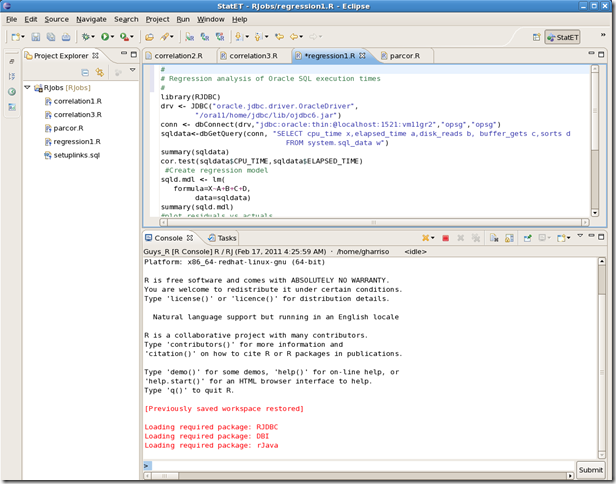
RJDBC hooks up pretty much any JDBC datasource into R, while ROracle uses native libraries to mediate the connection.  RJDBC is probably easier to start with, but ROracle can be installed pretty easily, provided you create some client libary entries.  So for me,  after downloading the ROracle package, my install looked something like this (run it as root):

cd $ORACLE_HOME/bin
genclntsh
genclntst

R CMD INSTALL --configure-args='--enable-static' /root/Desktop/ROracle_0.5-9.tar.gz

It was pretty obvious right away that RJDBC was much slower than ROracle.  Here’s a plot of elapsed times for variously sized datasets:

The performance of RJDBC degrades fairly rapidly as the size of the data being retrieved from Oracle increases,  and would probably be untenable for very large data sets. 

The RJDBC committers do note that RJDBC performance will not be optimal:

The current implementation of RJDBC is done entirely in R, no Java code is used. This means that it may not be extremely efficient and could be potentially sped up by using Java native code. However, it was sufficient for most tasks we tested. If you have performance issues with RJDBC, please let us know and tell us more details about your test case.

The default array size used by RJDBC is only 10, while the default for Roracle is 500… could this be the explaination for the differences in performance?

You can’t change the default RJDBC fetch size (at least, I couldn’t work out how to), but you can change ROracle's.  Here’s a breakdown of elapsed time for RJDBC and Roracle using defaults, and for ROracle using a fetch size of 10:

As you can see, issue does not seem to be the array size alone.   I suspect the overhead of building up the data frame from the result set in RJDBC is where the major inefficiency occurs.  Increasing the array fetch size might reduce the impact of this, but the array fetch size alone is not the cause of the slow performance.    

Conclusion

The current implementation of RJDBC is easy to install and fairly portable, but doesn’t provide good performance when loading large data sets.   For now, ROracle is the better choice.   

Scripts:

Create test table (SQL)

scalability testing (R script)

Comparison of elapsed times and array size (R script).

Statistical analysis of Oracle performance data using R

R is without doubt the Open Source tool of choice for statistical analysis, it contains a huge variety of statistical analysis techniques – rivalled only by hugely expensive commercial products such as SAS and SPSS.   I’ve been playing with R a bit lately, and – of course – working with data held in Oracle.  In particular, I’ve been playing with data held in the Oracle dynamic performance views.

This post is a brief overview of installing R, connecting R to Oracle, and using R to analyse Oracle performance data.

Installing R

R can be install in linux as a standard package:

yum install R

On Windows, you may wish to use the Revolution R binaries:  http://info.revolutionanalytics.com/download-revolution-r-community.html.  I had a bit of trouble installing the 32-bit binaries on my system as they conflicted with my 64-bit JDBC.  But if you are 32-bit you might be OK.

The easiest way to setup a connection to Oracle in to install the RJDBC package.

[oracle@GuysOEL ~]$ R

R version 2.12.1 (2010-12-16)
Copyright (C) 2010 The R Foundation for Statistical Computing
ISBN 3-900051-07-0
Platform: x86_64-redhat-linux-gnu (64-bit)

<snip>

Type 'demo()' for some demos, 'help()' for on-line help, or
'help.start()' for an HTML browser interface to help.
Type 'q()' to quit R.

> install.packages("RJDBC")

Using the StatET Eclipse plug-in

I use a free eclipse plug-in called StatET.  It provides an editing environment and GUI console for the R system.  The configuration steps are a little laborious, but it has a online getting started module that guides you through the steps.  Once you have it installed, I doubt you’ll go back to the command line. 

You can get StatET at http://www.walware.de/goto/statet.  Using the eclipse environment is really handy if you’re going to use R with Oracle, since you can also use the free Toad for Eclipse extension to work on your SQLs.  Eclipse becomes a complete environment for both R and Oracle.

Getting data from Oracle into R

Once you’ve installed R, it’s pretty simple to get data out of Oracle and into R.   Here’s a very short snippet that grabs data from the V$SQL table:

   1: library(RJDBC)

   2:  

   3: drv <- JDBC("oracle.jdbc.driver.OracleDriver",

   4:                 "/ora11/home/jdbc/lib/ojdbc6.jar")

   5:  

   6: conn <- dbConnect(drv,"jdbc:oracle:thin:@hostname:1521: service","username","password")

   7: sqldata<-dbGetQuery(conn, "SELECT cpu_time cpu,elapsed_time ela,disk_reads phys,

   8:                                   buffer_gets bg,sorts sorts

   9:                              FROM V$SQL ")

  10: summary(sqldata)

Let’s look at that line by line:

Line	Comments
1	The library command loads the RJDBC module, which will provide connectivity to Oracle.
3	We create a driver object for the Oracle JDBC driver.  The second argument is the location of the Oracle JDBC jar file,  almost always $ORACLE_HOME/jdbc/lib/ojdbc6.jar.
6	Connect to the Oracle database using standard JDBC connections strings
7	Create an R dataset from the result set of a query.  In this case, we are loading the contents of the V$SQL table.
10	The R “summary” package provides simple descriptive statistics for each variable in the provided dataset.

Basic R statistical functions

R has hundreds of statistical functions,  in the above example we used “summary”, which prints descriptive statistics.  The output is shown below;  mean, medians, percentiles, etc:

Correlation

Statistical correlation reveals the association between two numeric variables.  If two variables always increase or decrease together the correlation is 1;  if two variables are absolutely random with respect of each other then the correlation tends towards 0.

cor prints the correlation between every variable in the data set:

cor.test calculates the correlation coefficient and prints out the statistical significance of the correlation, which allows you to determine if there is a significant relationship between the two variables.  So does the number of sorts affect response time?  Let’s find out:

The p-value is 0.19 which indicates no significant relationship – p values of no more than 0.05 (one chance in 20) are usually requires before we assume statistical significance.

On the other hand,  there is a strong relationship between CPU time and Elapsed time:

Plotting

plot prints a scattergram chart.  Here’s the output from plot(sqldata$ELA,sqldata$CPU):

Here’s a slightly more sophisticated chart using “smoothScatter”, logarithmic axes and labels for the axes:

Regression

Regression is used to draw “lines of best fit” between variables.  

In the simplest case, we use the “lm” package to create a linear regression model between two variables (which we call “regdata” in the example).  The summary function prints a summary of the analysis:

This might seem a little mysterious if your statistics is a bit rusty, but the data above tells us that there is a significant relationship between elapsed time (ELA) and physical reads (PHYS) and gives us the gradient and Y axis intercept if we wanted to draw the relationship.   We can get R to draw a graph, and plot the original data by using the plot at abline functions:

Testing a hypothesis

One of the benefits of statistical analysis is you can test hypotheses about your data.  For instance, what about we test the until recently widely held notion that the buffer cache hit rate is a good measure of performance.  We might suppose if that were true that SQL statements with high buffer cache hit rates would show smaller elapsed times than those with low buffer cache hit rates.  To be sure, there are certain hidden assumptions underlying that hypothesis, but for the sake of illustration let’s use R to see if our data supports the hypothesis.

Simple correlation is a fair test for this, all we need to do is see if there is a statistically signifcant correlation between hit rate and elapsed time.  Here’s the analysis:

The correlation is close to 0, and the statistical significance way higher than the widely accepted .05 threshold for statistical significance.  Statements with high hit ratios do not show statistically signficantly lower elasped times that SQLs with low hit ratios.

Conclusion

There’s tons of data in our Oracle databases that could benefit from statistical analysis – not the least the performance data in the dynamic performance views, ASH and AWR.  We use statistical tests in Spotlight on Oracle to extrapolate performance into the future and to set some of the alarm thresholds.  Using R,  you have easy access to the most sophisticated statistical analysis techniques and as I hope I’ve shown, you can easily integrate R with Oracle data.

Correlation probability in Oracle

Being at the OReilly Strata conference has re-energized my inner statistic geek,  so I thought I’d share a PL/SQL package I some  years ago to calculate the probability associated with correlation coefficients calculated by Oracle.

Correlation is a statistical measure of the association between two variables.  Oracle introduced direct support for correlation in the SQL language from at least 10g (may have even been 9i).  So we can write SQL statements that calculate correlation.  So for instance,  this statement generates the correlation between the number of sorts and the elapsed times of SQL statements still cached in the SQL area:

The correlation coefficient “r” will be 1 if the two variables always increase or decrease together and –1 if one variable always increases as the other decreases.  A correlation coefficient of .33 probably represents some relationship, but anyone who has done statistics knows that you should calculate the statistical significance – chance that the result did not arise from chance – before making assertions.

Oracle doesn’t report correlation probabilities, so I implemented the formula to calculate the probability in  a PLSQL package.  It’s here.

If you pass the correlation coefficient and the number of samples (rows input to the CORR function) into the CORR_PROG_PKG.PROB_R function then it will show you the probability associated with that correlation.  So below we see the probability that this correlation is due to random fluctuation is effectively 0 (down to 4 significant figures):

Generally if the probability is less than .05 or .01 (one in 20 or 1 in 100 respectively) , then we would refer to the correlation as being statistically significant and that the two variables are related.  So we would be justified in claiming there was a relationship between sorts and elapsed time.

Just for kicks,   let’s use this technique to test the hypothesis that the Buffer Cache Hit ratio is a reliable indicator of performance.  Here’s the result:

The correlation is very low and the probability that there is no association is very high – way above the .05 probability.  In other words, in this database there is no statistically significant relationship between the elapsed time of an SQL and it’s buffer cache hit rate!

Working with Cassandra 0.7

In this post,  I experimented with inserting data from Oracle into Cassandra column families using Hector.  Unfortunately, that code isn’t compatible with the latest Cassandra 0.7 release, so I had to rework it.  The new version uses the addInsertion method of the Mutator object and while not totally intuitive didn’t take long to get working.  Here are the key changes:

   1: private static void insertSales(Connection oracleConn, Keyspace keyspace,

   2:         String cfName) throws SQLException {

   3:     int rows = 0;

   4:     ColumnPath cf = new ColumnPath(cfName);

   5:     Statement query = oracleConn.createStatement();

   6:  

   7:     String sqlText = "SELECT cust_id, cust_first_name,  cust_last_name, prod_name, "

   8:             + "           SUM (amount_sold) sum_amount_sold,sum(quantity_sold) sum_quantity_sold "

   9:             + "          FROM sh.sales    "

  10:             + "          JOIN sh.customers USING (cust_id) "

  11:             + "          JOIN sh.products  USING (prod_id)  "

  12:             + "         GROUP BY cust_id, cust_first_name,  cust_last_name,  prod_name "

  13:             + "         ORDER BY cust_id, prod_name ";

  14:     ResultSet results = query.executeQuery(sqlText);

  15:     int rowCount = 0;

  16:     int lastCustId = -1;

  17:     while (results.next()) { // For each customer

  18:         Integer custId = results.getInt("CUST_ID");

  19:         String keyValue = custId.toString();

  20:  

  21:         if (rowCount++ == 0 || custId != lastCustId) { // New Customer

  22:             String custFirstName = results.getString("CUST_FIRST_NAME");

  23:             String custLastName = results.getString("CUST_LAST_NAME");

  24:             System.out.printf("%s %s\n", custFirstName, custLastName);

  25:             // Create a supercolumn for customer details (first, lastname)

  26:             Mutator<String> mutator = HFactory.createMutator(keyspace,

  27:                     stringSerializer);

  28:             mutator.addInsertion(keyValue, cfName, HFactory

  29:                     .createSuperColumn("CustomerDetails", Arrays

  30:                             .asList(HFactory.createStringColumn(

  31:                                     "customerFirstName", custFirstName)),

  32:                             StringSerializer.get(), StringSerializer.get(),

  33:                             StringSerializer.get()));

  34:             mutator.addInsertion(keyValue, cfName, HFactory

  35:                     .createSuperColumn("CustomerDetails", Arrays

  36:                             .asList(HFactory.createStringColumn(

  37:                                     "customerLastName", custLastName)),

  38:                             StringSerializer.get(), StringSerializer.get(),

  39:                             StringSerializer.get()));

  40:  

  41:             mutator.execute();

  42:         }

  43:         // Insert product sales total for that customer

  44:         String prodName = results.getString("PROD_NAME");

  45:         Float SumAmountSold = results.getFloat("SUM_AMOUNT_SOLD");

  46:         Float SumQuantitySold = results.getFloat("SUM_QUANTITY_SOLD");

  47:         // Supercolumn name is the product name

  48:         Mutator<String> mutator = HFactory.createMutator(keyspace,

  49:                 stringSerializer);

  50:         mutator.addInsertion(keyValue, cfName, HFactory.createSuperColumn(

  51:                 prodName, Arrays.asList(HFactory.createStringColumn(

  52:                         "AmountSold", SumAmountSold.toString())),

  53:                 StringSerializer.get(), StringSerializer.get(),

  54:                 StringSerializer.get()));

  55:         mutator.addInsertion(keyValue, cfName, HFactory.createSuperColumn(

  56:                 prodName, Arrays.asList(HFactory.createStringColumn(

  57:                         "QuantitySold", SumQuantitySold.toString())),

  58:                 StringSerializer.get(), StringSerializer.get(),

  59:                 StringSerializer.get()));

  60:         mutator.execute(); 

  61:         lastCustId = custId;

  62:         rows++;

  63:     }

  64:     System.out.println(rows + " rows loaded into " + cf.getColumn_family());

  65: }

The reason why I wanted to do this was to play with Cassandra using our (relatively) new Toad for Cloud Databases Eclipse client.  Toad for Cloud Databases lets you work with non-relational datasources such as Cassandra, HBase, SimpleDB, etc, using SQL.   

Here’s how it works.  We select the column family we want to map from the Cassandra server:

That column family contains data loaded from both the Oracle CUSTOMER and SALES tables.   Toad recognizes that the data in that single column family is best represented by two normalized tables,  and gives us the opportunity to specify the names for the primary and foreign keys.  We can also rename the “tables” (more like views really) that Toad will create:

The resulting tables look similar to the tables that we originally loaded from Oracle, and we can issue SQL queries against them just as we could have with Oracle.  The queries get translated from SQL to thrift calls against the underlying Cassandra Server:

I definitely find it easier to issue SQL than write a 200 line Java program to do the same thing!  Of course, I'm not much of a Java programmer, but at a minimum having Toad to query the Cassandra data is invaluable when checking to see that your program did was it was intended to do 

Accelerating Oracle database performance with SSD

I was recently asked to provide advice on how best to accelerate Oracle database performance with flash SSD.   In this post I’ll attempt to outline some thoughts on that.

There’s some thinking that SSD will soon replace spinning disk altogether - we just have to wait for the price to come down.  However, I’m not so sure that this complete replacement is likely to occur in the immediate future.   There are two competing forces at work:

• The economies of “big data”, which drive us to reduce the cost per unit of storage ($$/TB):   magnetic disk costs only about 5% of the cost of a high end SSD per terabyte.
• The economies of high IO throughput, in which we are motivated to reduce the cost of providing a given IO rate.  SSD (PCi flash) can generate IO rates at 1/20th of the cost of magnetic disks.

These two competing economies are not likely to change in the immediate future:  magnetic disk can store large amounts of data much more cheaply than SSD;  SSD can deliver very high IO rates more cheaply than magnetic disk.  For most databases, it will not be cost effective to place the entire database on SSD – the best outcome will be obtained when we place parts of the database on SSD and some on magnetic disk.

SSD Performance basics

I’ve posted in the past on how SSD works with the Oracle flash cache,  and I’ve presented on SSD performance at OOW.  You might like to review those items.  However,  here’s a quick review of the basics:

• All flash drives offer pretty good read performance – say 25 microseconds for a single page read
• When inserting data into an empty page, performance is slower, but not awful – around 250 microseconds
• In order to update an existing page, a block erase is required – much, much slower – maybe 2000 microseconds

Enterprise SSD vendors - Fusion IO, Virident, etc - all have sophisticated algorithms to avoid the write penalty associated with SSD block erase operations.  Amongst other techniques, they will maintain a pool of unused blocks.  When a page needs to be updated it will be marked as invalid in the original location and moved to one of these blocks.  Later on, garbage collection routines will clear up the invalid entries.  The result is that updates don't always have to incur the high overhead of block erase operations.

Nevertheless, you want to avoid placing write intensive files on a flash disk, because as the disk fills up with modified blocks - and especially if the write rate exceeds the garbage collection capabilities - you might see the disk slow down dramatically.

To summarize:

Flash-based disks perform reads much faster than writes, and can suffer from performance degradation if subjected to intensive sustained write operations.

Options for SSD deployment on Oracle

Given the performance characteristics of SSD,  how best to use SSD to boost Oracle performance?  There are a few options:

• Put the entire database on SSD
• Place selected segments on SSD
• Use the 11GR2 flash cache
• Put temporary tablespace on SSD
• Put the redo logs on SSD

Let’s look at each of these in turn:

Put the entire Database on SSD

This works great – if you can afford it.  For most databases the cost of putting it all on SSD is too high.  Placing data that is rarely accessed on SSD is not very cost effective, because you are paying a high cost per GB, but not getting any benefit from the relatively cheap IO rates. 

Place selected segments on SSD

This is probably the best option if you don’t have enough SSD for the entire database, but it does require a bit of configuration.   We identify the segments with the most IO,  perhaps using a query on V$SEGMENT_STATISTICS:

 

We are looking for object that have a high read/write ratio, contribute to a significant number of reads, and are small enough to fit on our SSD.   We create a tablespace on SSD, then move these objects to that tablespace.

If our most read intensive tables are massive, then they might not fit on the SSD.  In this case we could consider partitioning them and placing the hottest partitions on SSD.  

Use the 11GR2 flash cache

If you have 11GR2 and are on a compatible platform (Solaris or Oracle Enterprise Linux), then you can setup the Oracle DB flash cache.  This is absolutely the easiest option – all you need to do is set a few parameters and bounce the database.  The flash cache automatically caches the hottest blocks and usually provides an excellent performance improvement.

The improvement is not as significant as moving objects directly onto flash storage, since there still has to be magnetic disk IO getting things on and off.  Also, the architecture tends to create a lot of writes to the SSD, which can challenge garbage collection.  The chart below sums up a typical outcome – a huge boost from the flash cache, but not as big a boost as we could get by putting objects directly on SSD:

Put temporary tablespace on SSD

Temporary tablespace IO (from sorts and hash operations) can sometimes be the most significant form of database IO, and often the entire temporary tablespace will fit on the SSD.  So should we consider putting temporary tablespace on the SSD?

I’m a bit reluctant to do this:  by definition temporary tablespace IO is equal parts reads and writes, and since we are motivated to avoid write IO to the SSD, this seems like a dubious option.  However, if your performance is absolutely dominated by temp tablespace IO and your SSD is tolerant of high write rates (eg has excellent garbage collection,etc) then it might be worth trying.  After all,  the SSD will definitely speed up the read side of temporary tablespace IO, even if the write IO does not get a significant boost. 

Put redo logs on SSD

Although redo logs are very IO intensive, it’s almost all write IO and therefore this is probably not the best option.   During sustained writes the Garbage Collection will probably break down and the disk might not end up performing that much better than a spinning disk.  I'd not recommend this. 

Conclusions

You can use SSD to boost database performance even if you don’t have enough for the entire database.  Best options are:

1. Place segments with high read but low write rates directly on SSD
2. Use the SSD with the 11GR2 database flash cache (if you are on OEL or Solaris)
3. If temporary segment IO is absolutely your bottleneck – but only then – consider placing the temporary tablespace on SSD.

I don’t think using SSD for redo logs is a good idea.  The high rates of sustained sequential write IO is not the ideal type of IO for SSD.