Joining V$PQ_TQSTAT to PLAN_TABLE output

When optimizing parallel execution, we have a couple oof sources of information, perhaps most importantly:

• The parallel execution plan as revealed by EXPLAIN PLAN and DBMS_XPLAN
• The data flows between each set of parallel processes as revealed by V$PQ_TQSTAT

 
The execution plan allows us to identify any serial bottlenecks in an otherwise parallelized plan, usually revealed by PARALLEL_FROM_SERIAL or S->P values in either the OTHER_TAG of the PLAN_TABLE or in the IN-OUT column of DBMS_XPLAN.

V$PQ_TQSTAT shows us the number of rows sent between each sets of parallel slaves. This helps determine if the work is being evenly divided between parallel slaves. Skew in the data can result in some slaves being over worked while others are underutilized. The result is that the query doesn’t scale well as parallel slaves are added.

Unfortunately, V$PQ_TQSTAT output is only visible from within the session which issued the parallel query and only for the most recent query executed. This limits its usefulness in a production environment, but it is still invaluable when tuning parallel queries.
It’s quite hard to correlate the output of DBMS_XPLAN and V$TQ_STAT so I wrote a script that tries to merge the output of both. It generates a plan for the last SQL executed by the session, and then joins that to the V$PQ_TQSTAT data. This is a little tricky, but I think the resulting script will generate useful output in a reasonably wide range of scenarios.

You can get the scrip here: tq_plan.sql. Your session will need access to the V$SQL_PLAN, V$SESSION and V$PQ_TQSTAT views.

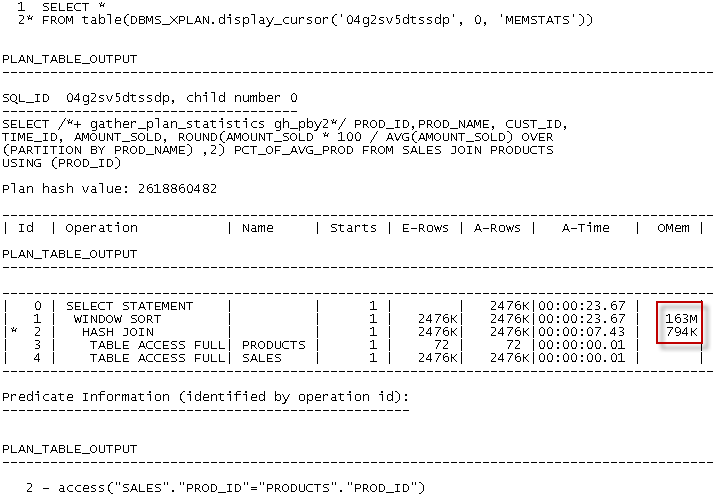
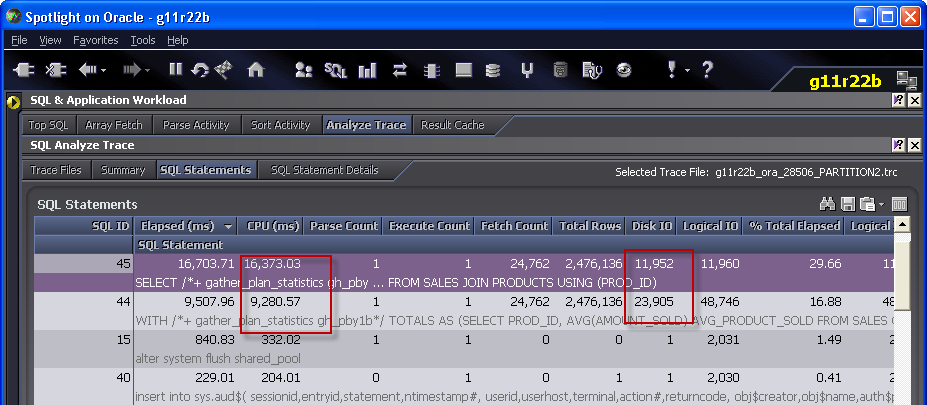
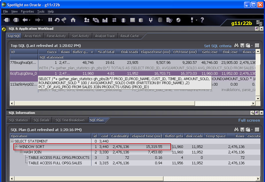
Here’s some example output:

 

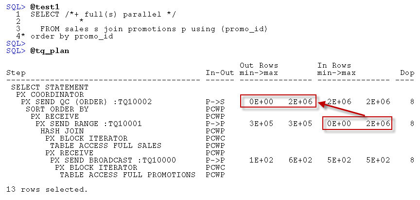
For each P->P, S->P or P->S step, the script shows the degree of parallelism employed ("Dop"), and the maximum and minimum rows processed by slaves. "Out Rows" represents the rows pushed from the first set of slaves, “In Rows” represents the number received by the next step. The highlighted portions of the above output reveal that this query is not parallelizing well: some slaves are processing 2 million rows, while others are processing none at all.

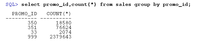
The reason this plan parallelizes so badly is that the PROMO_ID is such a skewed column.  Almost all the PROMO_IDs are 999 ("No promotion") and so parallelizing the ORDER_BY PROMO_ID is doomed:

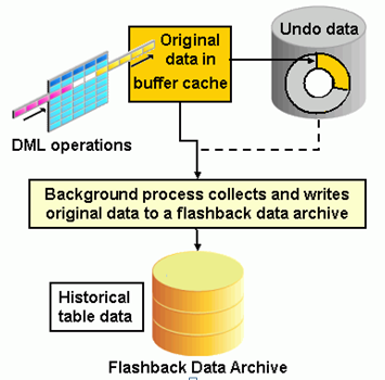
When we parallelize an ORDER BY, we allocate rows for various value ranges of the ORDER BY column to specific slaves.  For instance, in this diagram we see a parallelized ORDER BY on customer name; surnames from A-K are sent to one slave for sorting and surnames from L-Z sent to the other:

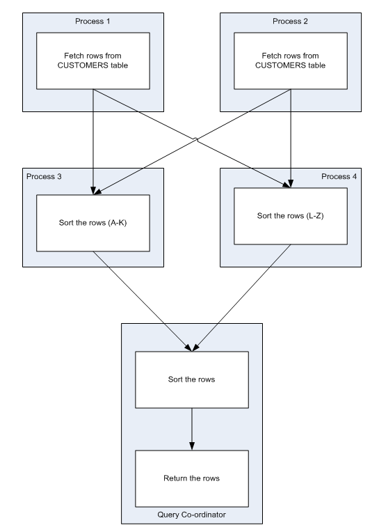
(This diagram is from Chapter 13 of Oracle Performance Survival Guide - ETA October 2009)

That approach works unless the rows are very skewed such as in our example - all 2 million of the "no promotion" rows go to a single slave which has to do virtually all of the work.

Anyway,  the v$pq_tqstat view, despite it's limitations, is the best way to analyze this sort of skew.  By linking the V$PQ_TQSTAT output to specific plan steps, hopefully my script will help you understand it's output.

PARTITION BY versus GROUP BY

 Here’s some more research that I did for the book that didn’t make make the final content.  It's a bit esoteric but interesting. 

In some circumstances you can use PARTITION BY to avoid doing a self-join to a GROUP BY subquery. However, although the PARTITION BY avoids duplicate reads of the table – usually a good thing – it won’t always lead to better performance.

For instance, if I want to create a report that compares each sale value to the average sale value for the product, I might join the sales data to a subquery with a GROUP BY product_id:

WITH /*+ gather_plan_statistics gh_pby1*/

     totals AS (SELECT prod_id,

                   AVG(amount_sold) avg_product_sold

                  FROM sales

                 GROUP BY prod_id)

SELECT prod_id, prod_name, cust_id, time_id, amount_sold,

       ROUND(amount_sold * 100 / avg_product_sold,2) pct_of_avg_prod

  FROM sales JOIN products USING (prod_id)

  JOIN totals USING (prod_id);

Of course, that approach requires two full scans of the SALES table (I used an expanded non-partitioned copy of the SH.SALES table from the Oracle sample schema). If we use the PARTITION BY analytic function we can avoid that second scan:

SELECT /*+ gather_plan_statistics gh_pby2*/

       prod_id,prod_name, cust_id, time_id, amount_sold,

       ROUND(amount_sold * 100 /

            AVG(amount_sold) OVER (PARTITION BY prod_name)

       ,2) pct_of_avg_prod

  FROM sales JOIN products USING (prod_id) ;

You’d expect that avoiding two scans of SALES would improve performance. However, in most circumstances the PARTITION BY version takes about twice as long as the GROUP BY version. Here’s some output from Spotlight’s analyse trace module – you can get some of the same information from tkprof if you don’t have Spotlight:

Notice how the version that uses the PARTITION BY clause has less logical IO but more physical IO. You might be thinking that this is something to do with buffer cache contents, but actually it’s a directly related to the WINDOW SORT Step that is characteristic of the analytic operation. You can see this in Spotlight when you look at the plan:

If you don’t have Spotlight, then you could see the same thing in tkprof, but you have to look closely at the step tags:

Analytic functions tend to be very memory intensive. The GROUP BY solution reads the SALES table twice, which requires some extra IO, but the PARTITION BY solution needs much more PGA memory. The default PGA allocation mechanisms – which limit the amount of memory available to individual processes and workeaas to a fraction of the overall PGA Aggregate Target- didn’t allocate enough memory for the operation to complete in memory and hence temporary segment IO resulted. As is so often the case, temporary segment IO overhead exceeded the datafile read overhead.

We can see how much memory was required by using DBMS_XPLAN.DISPLAY_CURSOR, looking at the V$SQL_PLAN entries or – if we have it – Spotlight:

To get it from DBMS_STATS, we could use the MEMSTATS option and provide the SQL_ID from V$SQL:

The memory wanted isn’t that much – only 163M – a trivial amount in this day and age. This database was running Automatic Memory Management (AMM) with a memory target of about 1.5GB. Oracle didn’t increase the PGA aggregate target even after I’d run this query (badly) several times, but still there was about 450M of PGA which should have been enough. Unfortunately, a single session cannot use all of the PGA target – under 1GB only 200M is available to a single serial session and only half that to a single work area.

In this circumstance I would probably be well advised to opt out of Automatic workarea management and set my own amount of sort memory: something like this:

ALTER SESSION SET workarea_size_policy = manual;

ALTER SESSION SET sort_area_size = 524288000;

(Jonathan lewis has reported a bug in this –see http://jonathanlewis.wordpress.com/2008/11/25/sas-bug/)

Once I do that, the temporary segment IO involved in the PARTITION BY reduces remarkably. However, it’s still slower than the GROUP BY.

The IO for the PARTITION BY is now much less than for the GROUP BY, but the CPU for the PARTITION BY is still much higher. Even when there is lots of memory, PARTITION BY – and many analytical functions – are very CPU intensive. Here we see that even without the temporary segment IO, the WINDOW SORT is the most expensive operation:

I used to think that analytic functions – by avoiding duplicate table reads – offered a performance solution to certain problems. However the more I use them the more often I find that the CPU and memory cost of the analytic function is greater than the IO savings that it enables.

So.... the moral of the story: Analytic functions are very powerful and allow you to improve the clarity and simplicity of a lot of complex SQLs. And there are definitely some things that can only be done in SQL if you use an analytic function solution. However, they are resource intensive – most notably on memory, but also on CPU. In particular, make sure that you don’t inadvertently cause SQL performance to degrade when you move to an analytic function solution because you caused temporary segment IO.

Flashback Data Archive performance (pt 1)

I did some research on Flashback Data Archive (FBDA) for my upcoming Oracle performance book, but decided not to include it in the book due to space limitations and because not many people are using FBDA just yet.

FBDA – also called Total Recall - is described by Oracle like this:

Overview

Flashback Data Archive provides the ability to automatically track and store all transactional changes to a record for the duration of its lifetime. This feature also provides seamless access to historical data with "as of" queries. It provides flashback functionality for longer time periods than your undo data. You can use Flashback Data Archive for compliance reporting, audit reports, data analysis and decision support.

http://www.oracle.com/technology/obe/11gr1_db/security/flada/flada.htm

Sounds good, but from my brief tests you pay a very high price for this functionality. Also, it looks like the background processing has been changed to foreground processing in 11.0.6.   In 11.0.6, it's the FBDA background process that populates the FBDA tables, but in 11.0.7 this is done by the session that issues the DML.

Let’s review FBDA set up first. Create a tablespace and a data archive:

CREATE TABLESPACE fb_arc_ts1 DATAFILE

'/oradata/g11r22a/fb_arc1.dbf' SIZE 1024 M AUTOEXTEND OFF;

DROP FLASHBACK ARCHIVE fb_arc1;

/* Create the flashback archive */

CREATE FLASHBACK ARCHIVE DEFAULT fb_arc1

TABLESPACE fb_arc_ts1

QUOTA 1024 M

RETENTION 1 DAY;

Now we can mark a table for flashback archive:

ALTER TABLE fba_test_data FLASHBACK ARCHIVE;

DML statements run about the same time on a FBDA table, but COMMIT times go through the roof:

SQL> UPDATE fba_test_data

2 SET datetime = datetime + .01;

999999 rows updated.

Elapsed: 00:01:13.43

SQL>

SQL> COMMIT;

Commit complete.

Elapsed: 00:24:10.29

That’s right – 1 minute update, 24 minute commit time!! I’ve seen the same performance from DELETEs and INSERTs.

When the COMMIT occurs, Oracle runs recursive SQL to update the data archive. Here’s an example of one of the SQLs that runs (shown in Spotlight on Oracle's trace file viewer):

The statement above is the final in a sequence of at least 4 that are executed for every transaction.

In 11.0.6, there’s a bug in the FBDA SQL. The following SQL has a hint missing the “+” sign. Consequently the intended direct path inserts do not occur and - in some cases - free buffer waits can result:

The free buffer waits are a consequence of creating lots of new blocks for the DBWR to write to disk while at the same time pulling lots of blocks into the buffer cache from the source table.  If the DBWR can't write out to disk as fast as you are creating new blocks then the free buffer waits results.

FBDA will large transactions is therefore not snappy.  For short transactions the effect (at COMMIT time on 11.0.7) is less noticeable:

SQL> INSERT INTO fba_test_data d(id, datetime, data)

2 SELECT ROWNUM id,

3 SYSDATE - 1000 + DBMS_RANDOM.VALUE(1, 1000) datetime,

4 RPAD(SYSDATE - 1000 + DBMS_RANDOM.VALUE(1, 1000), 900,

5 'x')

6 data

7 FROM DUAL

8 CONNECT BY ROWNUM < 10;

9 rows created.

Elapsed: 00:00:00.48

SQL>

SQL> COMMIT;

Commit complete.

Elapsed: 00:00:00.53

The SQLs that FBDA generates are interesting case studies for SQL tuning – the use of hints in particular is interesting since it limits the ability of Oracle to respond to different volumes of changes with different SQL plans. I’ll post an analysis of the various SQLs issued in a future post.

For now, the clear lesson is to be very cautious when implementing FBDA – it definitely has some performance implications!

New Book, New blog

 

I'm not a very good blogger at the best of times.  I'm just unable to get beyond the first, draft second draft, review process that works OK for articles and books, but which is not what you want when blogging.  Over the last six months I've been even worse, since all my spare energy has been going into writing the Oracle Performance Survival Guide.  This book has been by far the most challanging yet rewarding writing effort in my career.  I set out to write a book that could stand alone as a single guide to Oracle performancecovering all aspects of Oracle performance management,  suitable for all levels of expertise and across all relevant disciplines.  So there's equal weight given to application and database design, SQL and PL/SQL tuning, contention management, memory optimization and disk tuning.

Anyway,  it's been quite an effort and I learned a lot while writing it.  But it's taken over my life!

The books going to be available probably around Oracle Open World in October.  You can pre-order it from Amazon.

Now that I'm over the biggest hump in getting the book together,  I thought I'd try to get back into occasional blogging.  I'd heard good things about SquareSpace and once I took a look I was hooked.  This thing is way ahead of what I was using and is great for total website management, not just blog publishing.  Therefore I'm shutting down my old blog at http://guyharrison.typepad.com/ and running everything from here.  Hopefully,  I'll be motivated to blog more often than in the past!

Oracle on Amazon AWS

Ever since Oracle announced support for Amazon AWS at OOW I’ve been eager to play around with it.  I finally found the time and here are my notes in case it helps anyone get going.

Using Amazon AWS in general is a big topic. 

Here's an article I wrote for ToadWorld on the topic:

Getting started with Oracle in the Amazon cloud