Next Generation Databases

My latest book Next Generation Databases is now available to purchase!   You can buy it from Amazon here, or directly from Apress here.  The e-book versions are not quite ready but if you prefer the print version you’re good to go.

I wrote this book as an attempt to share what I’ve learned about non-relational databases in the last decade and position these in the context of the relational database landscape that I’ve worked in all my professional life.  

The book is divided into two sections:  the first section explains the market and technology drivers that lead to the end of complete “one size fits all” relational dominance and describes each of the major new database technologies.   These first 7 chapters are:

• Three Database Revolutions
• Google, Big Data, and Hadoop  
• Sharding, Amazon, and the Birth of NoSQL
• Document Databases
• Tables are Not Your Friends: Graph Databases
• Column Databases
• The End of Disk? SSD and In-Memory Databases 

The second half of the book covers the “gory details” of the internals of the major new database technologies.  We look at how databases like MongoDB, Cassandra, HBase, Riak and others implement clustering and replication, locking and consistency management, logical and physical storage models and the languages and APIs provided.  These chapters are: 

• Distributed Database Patterns 
• Consistency Models 
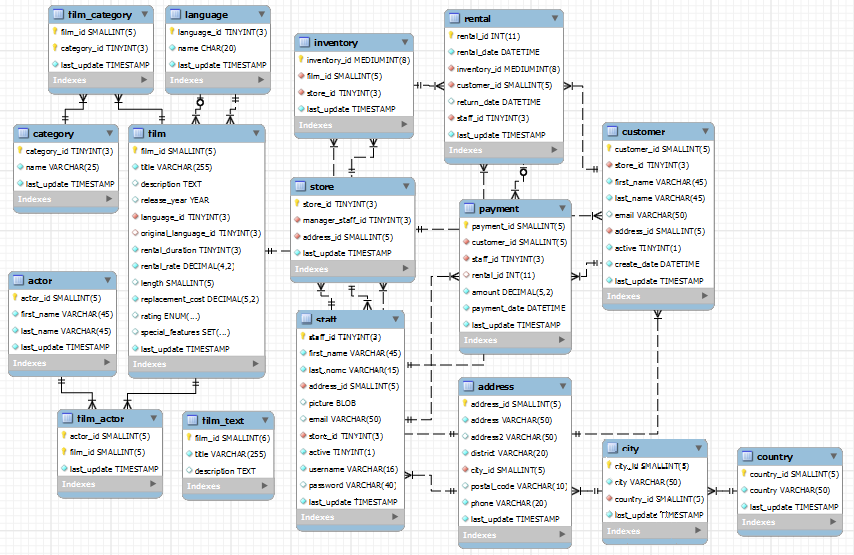
• Data Models and Storage 
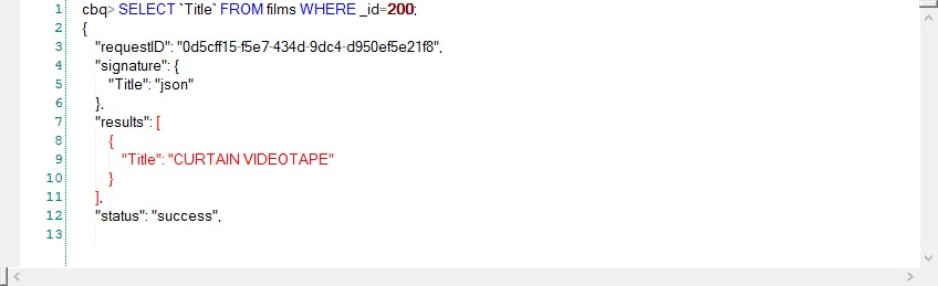
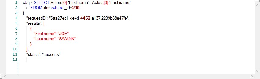
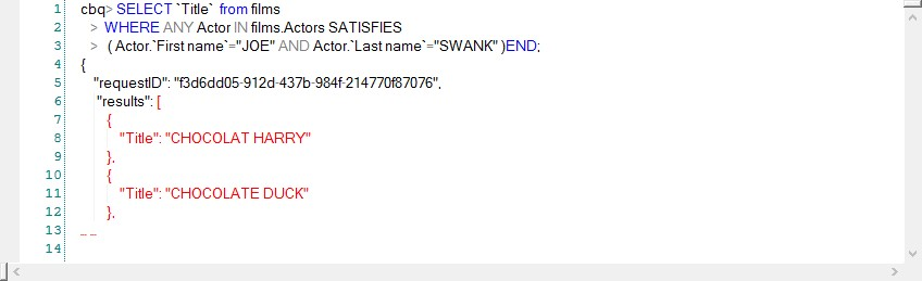
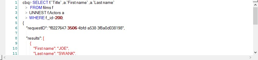
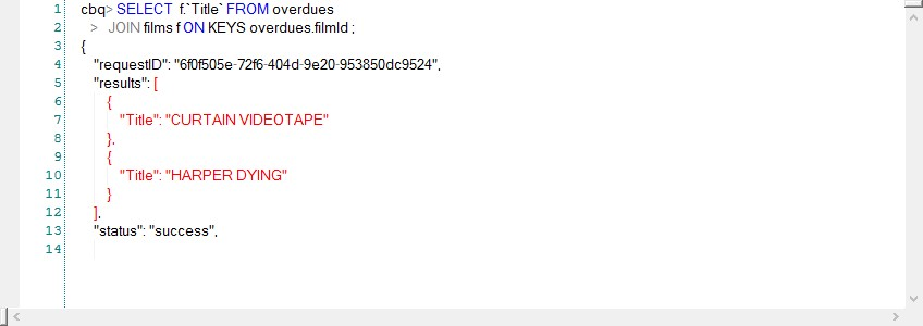
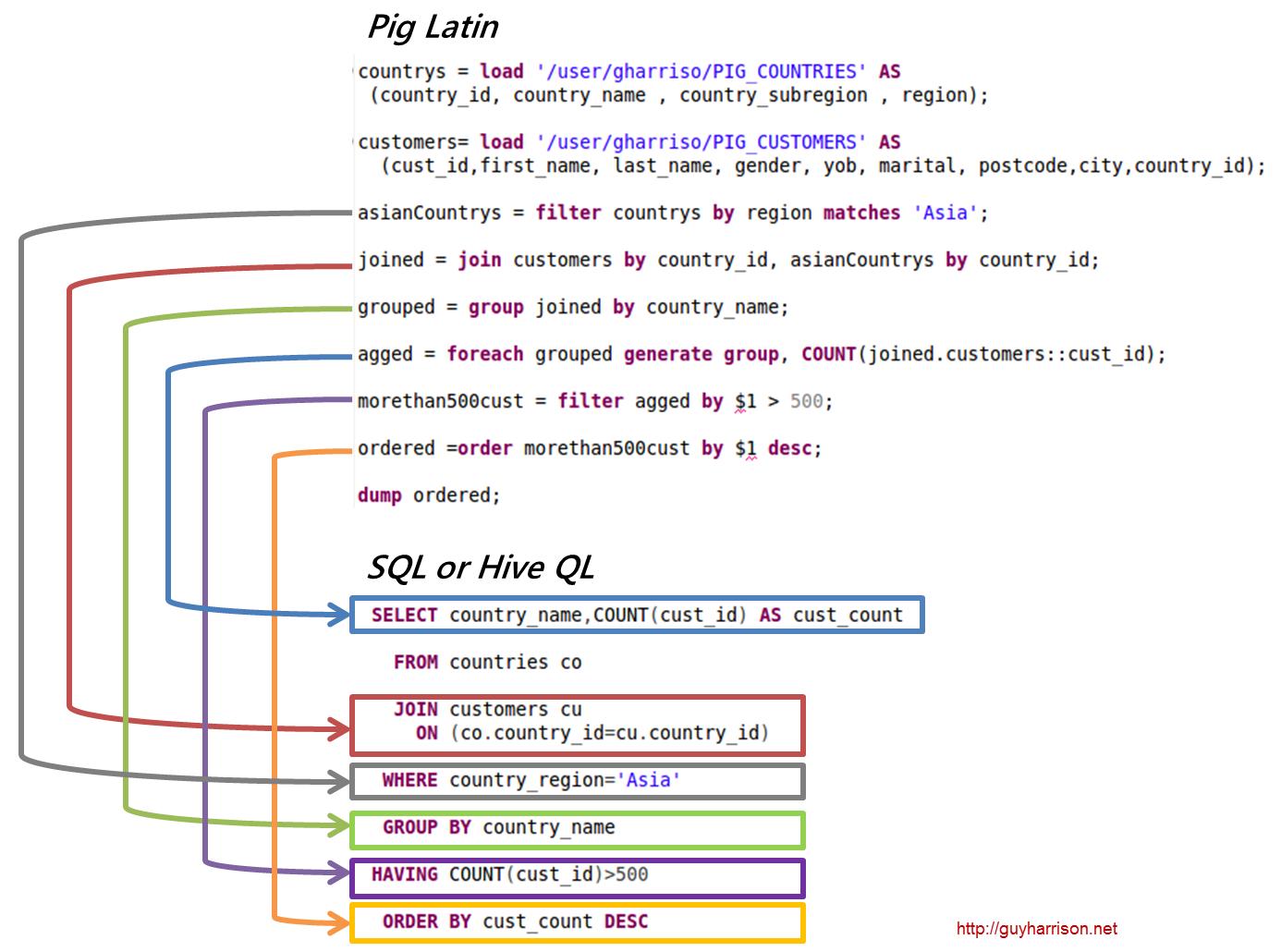
• Languages and Programming Interfaces

The final chapter speculates on how databases might develop in the future.  Spoiler alert: I think the explosion of new database technologies over the last few years is going to be followed by a consolidation phase, but there’s some potentially disruptive technologies on the horizon such as universal memory, blockchain and even quantum computing. 

The relational database is a triumph of software engineering and has been the basis for most of my career.  But the times they are a changing and speaking personally I’ve really enjoyed learning about these new technologies.  I learned a lot more about the internals of the newer database architectures while writing the book and I’m feeling pretty happy with the end result.   As always I’m anxious to engage with readers and find out what you guys think!

Vector clocks

 

Once of the concepts I found difficult initially when looking at non-relational systems is the concept of the vector clock.  Some databases – like Cassandra - use timestamps to work out which is the “latest” transaction. If there are two conflicting modifications to a column value, the one with the highest timestamp will be considered the most recent and the most correct.

Other Dynamo systems use a more complex mechanism known as a vector clock. The vector clock has the advantage of not requiring clock synchronization across all nodes, and helps us identify transactions that might be in conflict.

Despite its name, the vector clock does not include any timestamps. Rather it is composed of a set of counters. These counters are incremented when operations complete, in a similar way to the traditional System Change Number pattern that we are familiar with from relational systems like Oracle. The set contains one counter for each node in the cluster. Whenever an operation occurs on a node, that node will increment its own counter within its vector clock. Whenever a node transmits an operation to another node it will include its vector clock within the request. The transmitted vector clock will include the highest counter for the transmitting node as well is the highest counters from other nodes that the transmitting node has ever seen.

When a node receives possibly conflicting updates from other nodes, it can compare the vector clocks to determine the relative sequencing of the requests. There is a defined set of vector clock operations that can tell if:

• The two vector clocks come from nodes that are completely in sync
• One node is “out of date” with respect of the other node
• The clocks are “concurrent” in that each node has some information that is more up to date than the other node. In this case we can’t choose which update is truly the more correct.

Vector clocks are notoriously difficult to understand, though the underlying algorithm is really quite simple. The diagram below shows an example of three vector clocks incrementing across three nodes. The algorithm is somewhat simplified to improve clarity

 

In the example the vector clocks start out set to 0 for all nodes (1). Updates to nodes from external clients caused the nodes to increment their own element of the vector clock (2). When these changes are propagated to other nodes, the receiving node updates its vector clock and merges the vector clocks from the other nodes (3). Event (H) occurs when node 2 receives the vector clock (F) from node 1 and (G) from node 3 (4). Each of these vector clocks contain elements higher than the other - vector clock F has the higher value for node 1, while vector clock G has the higher value for node 3. There is no way for node 2 to be sure which of the two vector clocks represent the most up-to-date data - each of the sending nodes “knows” something that the other node does not, and consequently it’s not clear which of the two nodes “knows” best.

For those of us from the world of strictly consistent databases like Oracle, think of the vector clock as a set of System Change Numbers from each system.  We examine the SCNs from each node to see if there are nodes that might not have seen all the changes that have been recorded on another node.

The Vector clock in above us that Version G and Version F are conflicting – each contains information from unique updates that could both contain important information. What then, is the system to do? Here are some of the options:

• Revert to last write wins: two updates are unlikely to have occurred at the exact same nanosecond, so one will have a higher timestamp value. We could decide that the highest timestamp “wins”.
• Keep both copies, and require that the application or the user resolve the conflict.
• Somehow merge the data. This is the approach taken by the original Dynamo which managed Amazon’s shopping cart. If there are two conflicting shopping carts they are merged and the worst that can happen (from Amazon’s point of view) is that you buy some things twice. Another merge can occur with things like counters: rather than having one counter increment overwrite another, we can deduce that both operations wanted to increment the counter and increment it twice. A special class of data types: Conflict-Free Replicated Data Type (CRDT) exist that allow these sort of merges to be predefined.

There are advocates for the vector clock – such as the architects of Riak - , and advocates for the timestamp system used in Cassandra. Neither party disagree about the concrete implications of the two approaches: they differ on the desirability of the consequences. Last Write Wins represents a simpler model for the application developer and administrator, Vector clocks allow for conflicts to be identified but which must then be resolved.   In a later post I’ll give an example of how you programmatically resolve conflicts in Riak.

Exploring CouchBase N1QL

Couchbase recently announced Non-first Normal Form Query Language (N1QL) – pronounced “Nickel” – a virtually complete SQL language implementation for use with document databases, and implemented within the Couchbase server 4.0.

I recently took a quick look. 

Most of the examples use the sample films documents shown below (this is the same sample data we created for MongoDB in this post):

N1QL allows us to perform basic queries to retrieve selected documents or attributes of selected documents:

N1QL allows us to access nested documents within the JSON structure using array notation. So for instance in the example below Actors[0] refers to the first nested document within the actors array:

We can query for subdocuments which match a search criteria using WHERE ANY syntax:

The UNNEST command allows embedded documents to be “joined” back to the parent document. So here we get one result for each Actor who starred in film 200, with the film title included in the results:

The UNNEST command allows us to perform the equivalent of joins between parent and children documents where the child documents are nested within the parent. N1QL also allows us to join across disparate documents, providing that one of the document collections contains a reference to the primary key in the other.

So for instance if we had a bucket of documents that contains the primary keys of “overdue” films in our imaginary (and by now definitely struggling) DVD store, then we can join that to the films collection to return just those films:

N1QL also contains DML statements allowing us to manipulate the contents of documents, and DDL statements allowing creation and modification of indexes.

N1QL is ambitious attempt to bring SQL into the world of document databases. It’s interesting to consider that as the same time that companies like CouchBase are introducing SQL support into their database, that companies like Oracle are introducing strong JSON support into their SQL-based database. It would seem that the two worlds are coming together.

Sakila sample schema in MongoDB

2018 Update:  You can download this and other sample schemas we use in dbKoda from https://medium.com/dbkoda/mongodb-sample-collections-52d6a7745908.

I wanted to do some experimenting with MongoDB, but I wasn’t really happy with any of the sample data I could find in the web.  So I decided that I would translate the MySQL “Sakila” schema into MongoDB collections as part of the learning process.   

For those that don’t know, Sakila is a MySQL sample schema that was published about 8 years ago.  It’s based on a DVD rental system.   OK, not the most modern data ever, but DVDs are still a thing aren’t they??

You can get the MongoDB version of Sakilia here.  To load, use unpack using tar zxvf sakilia.tgz then use mongoimport to load the resulting JSON documents.  On windows you should be able to double click on the file to get to the JSON.  

The Sakila database schema is shown below.  There are 16 tables representing a fairly easy to understand inventory of films, staff, customers and stores.

When modelling MongoDB schemas, we partially ignore our relational modelling experience – “normalization” is not the desired end state.   Instead of driving our decision on the nature of the data, we drive it on the nature of operations.  The biggest decision is which “entities” get embedded within documents, and which get linked.  I’m not the best person to articulate these principles – the O’Reilly book “MongoDB Applied Design Patterns” does a pretty good job and this presentation is also useful.

My first shot at mapping the data – which may prove to be flawed as I play with MongoDB queries – collapsed the 16 tables into just 3 documents:  FILMS, STORES and CUSTOMERS.   ACTORS became a nested document in FILMS, STAFF and INVENTORY were nested into STORES, while RENTALS and PAYMENTS nested into CUSTOMERS.   Whether these nestings turn out to be good design decisions will depend somewhat on the application.  Some operations are going to be awkward while others will be expedited.

Here’s a look at the FILMS collection:

Here is STORES:

And here is CUSTOMERS:

Looks like I have to fix some float rounding issues on customers.rentals.payments.amount .

The code that generates the schema is here.   It’s pretty slow, mainly because of the very high number of lookups on rentals and payments.  It would be better to bulk collect everything and scan through it but it would make the code pretty ugly.   If this were Oracle I’m pretty sure I could make it run faster but with MySQL SQL tuning is much harder.

Code is pretty straight forward.  To insert a MongoDB document we get the DBCollection, then create BasicDBObjects which we insert into the DBCollection.  To nest a documnet we create a BasicDBList and insert BasicDBObjects into it.  Then we add the BasicDBList to the parent BasicDBObject.  The following snippit illustrates that sequence.  It's mostly boilerplate code, with the only human decision being the nesting structure. 

   1: DBCollection filmCollection = mongoDb.getCollection(mongoCollection);

   2:  

   3: while (fileRs.next()) { // For each film

   4:  

   5:         // Create the actors document

   6:         BasicDBObject filmDoc = new BasicDBObject();

   7:         Integer filmId = fileRs.getInt("FILM_ID");

   8:         filmDoc.put("_id", filmId);

   9:         filmDoc.put("Title", fileRs.getString("TITLE"));

  10:         // Other attributes

  11:         BasicDBList actorList = getActors(mysqlConn, filmId);

  12:         // put the actor list into the film document

  13:         filmDoc.put("Actors", actorList);

  14:         filmCollection.insert(filmDoc); // insert the film

  15:  

  16:     }

Anyway, hopefully this might be of some use to those moving from MySQL to MongoDB.  Comments welcome!

Getting started with Apache Pig

If, like me, you want to play around with data in a Hadoop cluster without having to write hundreds or thousands of lines of Java MapReduce code, you most likely will use either Hive (using the  Hive Query Language HQL) or Pig.

Hive is a SQL-like language which compiles to Java map-reduce code, while Pig is a data flow language which allows you to specify your map-reduce data pipelines using high level abstractions. 

The way I like to think of it is that writing Java MapReduce is like programming in assembler:  you need to manually construct every low level operation you want to perform.  Hive allows people familiar with SQL to extract data from Hadoop with ease and – like SQL – you specify the data you want without having to worry too much about the way in which it is retrieved.  Writing a Pig script is like writing a SQL execution plan:  you specify the exact sequence of operations you want to undertake when retrieving the data.  Pig also allows you to specify more complex data flows than is possible using HQL alone.

As a crusty old RDBMS guy, I at first thought that Hive and HQL was the most attractive solution and I still think Hive is critical to enterprise adoption of Hadoop since it opens up Hadoop to the world of enterprise Business Intelligence.  But Pig really appeals to me as someone who has spent so much time tuning SQL.  The Hive optimizer is currently at the level of early rule-based RDBMS optimizers from the early 90s.  It will get better and get better quickly, but given the massive size of most Hadoop clusters, the cost of a poorly optimized HQL statement is really high.  Explicitly specifying the execution plan in Pig arguably gives the programmer more control and lessens the likelihood of the “HQL statement from Hell” brining a cluster to it’s knees.

So I’ve started learning Pig, using the familiar (to me) Oracle sample schema which I downloaded using SQOOP.   (Hint:  Pig likes tab separated  files, so use the --fields-terminated-by '\t' flag in your SQOOP job). 

Here’s a diagram I created showing how some of the more familiar HQL idioms are implemented in Pig:

Note how using Pig we explicitly control the execution plan:  In HQL it’s up to the optimizer whether tables are joined before or after the “country_region=’Asia’” filter is applied.  In Pig I explicitly execute the filter before the join.    It turns out that the Hive optimizer does the same thing, but for complex data flows being able to explicitly control the sequence of events can be an advantage. 

Pig is only a little more wordy than HQL and while I definitely like the familiar syntax of HQL I really like the additional control of Pig.