Getting started with Apache Pig

If, like me, you want to play around with data in a Hadoop cluster without having to write hundreds or thousands of lines of Java MapReduce code, you most likely will use either Hive (using the  Hive Query Language HQL) or Pig.

Hive is a SQL-like language which compiles to Java map-reduce code, while Pig is a data flow language which allows you to specify your map-reduce data pipelines using high level abstractions. 

The way I like to think of it is that writing Java MapReduce is like programming in assembler:  you need to manually construct every low level operation you want to perform.  Hive allows people familiar with SQL to extract data from Hadoop with ease and – like SQL – you specify the data you want without having to worry too much about the way in which it is retrieved.  Writing a Pig script is like writing a SQL execution plan:  you specify the exact sequence of operations you want to undertake when retrieving the data.  Pig also allows you to specify more complex data flows than is possible using HQL alone.

As a crusty old RDBMS guy, I at first thought that Hive and HQL was the most attractive solution and I still think Hive is critical to enterprise adoption of Hadoop since it opens up Hadoop to the world of enterprise Business Intelligence.  But Pig really appeals to me as someone who has spent so much time tuning SQL.  The Hive optimizer is currently at the level of early rule-based RDBMS optimizers from the early 90s.  It will get better and get better quickly, but given the massive size of most Hadoop clusters, the cost of a poorly optimized HQL statement is really high.  Explicitly specifying the execution plan in Pig arguably gives the programmer more control and lessens the likelihood of the “HQL statement from Hell” brining a cluster to it’s knees.

So I’ve started learning Pig, using the familiar (to me) Oracle sample schema which I downloaded using SQOOP.   (Hint:  Pig likes tab separated  files, so use the --fields-terminated-by '\t' flag in your SQOOP job). 

Here’s a diagram I created showing how some of the more familiar HQL idioms are implemented in Pig:

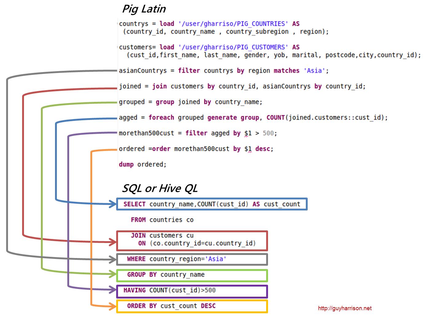
Note how using Pig we explicitly control the execution plan:  In HQL it’s up to the optimizer whether tables are joined before or after the “country_region=’Asia’” filter is applied.  In Pig I explicitly execute the filter before the join.    It turns out that the Hive optimizer does the same thing, but for complex data flows being able to explicitly control the sequence of events can be an advantage. 

Pig is only a little more wordy than HQL and while I definitely like the familiar syntax of HQL I really like the additional control of Pig.

Amazon Elastic Map Reduce (EMR), Hive, and TOAD

Since my first post on connecting to Amazon Elastic Map Reduce with TOAD, we’ve added quite a few features to our Hadoop support in general and our EMR support specifically, so I thought I’d summarize those features in this blog post

Amazon Elastic Map Reduce is a cloud-based version of Hadoop hosted on Amazon Elastic Compute Cloud (EC2) instance.  Using EMR, you can quickly establish a cloud based Hadoop cluster to perform map reduce work flows. 

EMR support Hive of course, and Toad for Cloud Databases (TCD)  includes Hive support, so let’s look at using that to query EMR data.

Using the Toad direct Hive client

TCD direct Hive connection support is the quickest way to establish a connection to Hive.  It uses a bundled JDBC driver to establish the connection.

Below we create a new connection to a Hive server running on EMR:

1. Right click on Hive connections and choose “Connect to Hive” to create a new Hive connection.
2. The host address is the “Master” EC2 instance for your EMR cluster.  You’ll find that on the EMR Job flow management page within your Amazon AWS console.  The Hive 0.5 server is running on port 10000 by default.
3. Specifying a job tracker port allows us to track the execution of our Hive jobs in EMR.  The standard Hadoop jobtracker port is 50030, but in EMR it’s 9600.
4. It’s possible to open up port 10000 so you can directly connect with Hive clients, but it’s a bad idea usually.  Hive has negligible built-in security, so you’d be exposing your Hive data.   For that reason we support a SSH mode in which you can tunnel through to your hadoop server using the keypair file that you used to start the EMR job flow.  The key name is also shown in the EMR console page, though obviously you’ll need to have an actual keypair file.

The direct Hive client allows you to execute any legal Hive QL commands.  In the example below, we create a new Hive table based on data held in an S3 bucket (The data is some UN data on homicide rates I uploaded).

Connecting Hive to the Toad data hub

It’s great to be able to use Hive to exploit Map Reduce using familiar (to me) SQL-like syntax.  But the real advantage of TCD for Hive is that we link to data that might be held in other sources – like Oracle, Cassandra, SQL Server, MongoDB, etc.

Setting up a hub connection to EMR hive is very similar to setting up a direct connection.  Of course you need a data hub installed (see here for instructions), then right click on the hub node and select “map data source”:

Now that the hub knows about the EMR hive connection, we can issue queries that access Hive and – in the same SQL – other datasources. For instance, here’s a query that joins homicide data in Hive Elastic Map Reduce with population data stored in a Oracle database (running as Amazonn RDS:  Relational Database Service).  We can do these cross platform joins across a lot of different types of database sources, including any ODBC compliant databases, any Apache Hbase or Hive connections, Cassandra, MongoDB, SimpleDB, Azure table services:

In the version that we are just about to release, queries can be saved as views or snapshots, allowing easier access from external tools of for users who aren’t familiar with SQL.   In the example above, I’m saving my query as a view.

 

Using other hub-enabled clients

TCD isn’t the only product that can issue hub queries.  In beta today, the Quest Business Intelligence Studio can attach to the data hub, and allows you to graphically explore you data using drag and drop, click and drilldown paradigms:

It’s great to be living in Australia – one of the lowest homicide rates!

If you’re a hard core data scientist, you can even attach R through to the hub via the RODBC interface.  So for instance, in the screen shot below, I’m using R to investigate the correlation  between population density and homicide rate.  The data comes from Hive (EMR) and Oracle (RDS),  is joined in the hub, saved as a snapshot and then feed into R for analysis.  Pretty cool for a crusty old stats guy like me (My very first computer program was written in 1979 on SPSS).

Comparing Hadoop Oracle loaders

Oracle put a lot of effort into highlighting the upcoming Oracle Hadoop Loader (OHL) at OOW 2011 – it was even highlighted in Andy Mendelsohn's keynote.  It’s great to see Oracle recognizing Hadoop as a top tier technology!

However, there were a few comments made about the “other loaders” that I wanted to clarify.  At Quest, I lead the team that writes the Quest Data Connector for Oracle and Hadoop (let’s call it the “Quest Connector”) which is a plug-in to the Apache Hadoop SQOOP framework and which provides optimized bidirectional data loads between Oracle and Hadoop.  Below I’ve outlined some of the high level features of the Quest Connector in the context of the  Oracle-Hadoop loaders.  Of course, I got my information on the Oracle loader from technical sessions at OOW so I may have misunderstood and/or the facts may change between now and the eventual release of that loader.  But I wanted to go on the record with the following:

• All parties (Quest, Cloudera, Oracle) agree that native SQOOP (eg, without the Quest plug-in) will be sub-optimal: it will not exploit Oracle direct path reads or writes, will not use partitioning, nologging, etc.   Both Cloudera and Quest recommend that if are doing transfers between Oracle and Hadoop that you use SQOOP with the Quest connector.
• The Quest connector is a free, open source plug in to SQOOP, which is itself a free, open source software product.  Both are licensed under the Apache 2.0 open source license.  Licensing for the Oracle Loader has not been announced, but Oracle has said it will be a commercial product and therefore presumably not free under all circumstances.   It’s definitely not open source.
• The Quest loader is available now (version 1.4), the Oracle loader is in beta and will be released commercially in 2012.
• The Oracle loader moves data from Hadoop to Oracle only.  The Quest loader can also move data from Oracle to Hadoop.   We import data into Hadoop from an Oracle database usually 5+ times faster than SQOOP alone.
• Both Quest and the Oracle loader use direct path writes when loading from Hadoop to Oracle.  Oracle do say they use OCI calls which may be faster than the direct path SQL calls used by Quest in some circumstances.   But I’d suggest that the main optimization in each case is direct path.
• Both Quest and the Oracle loader can do parallel direct path writes to a partitioned Oracle table.  In the case of the Quest loader, we create partitions based on the job and mapper ids.  Oracle can use logical keys and write into existing partitioned tables.  My understanding is that they will shuffle and sort the data in the mappers to direct the output to the appropriate partition in bulk.  They also do statistical sampling which may improve the load balancing when you are inserting into an existing table. 
• The Quest loader can update existing tables, and can do Merge operations that insert or updates rows depending on the existence of a matching key value.  My understanding is that the Oracle loader will do inserts only - at least initially.
• Both the Quest connector and the Oracle loader have some form of GUI.  The Oracle GUI I believe is in the commercial ODI product.  The Quest GUI is in the free Toad for Cloud Databases Eclipse plug-in.  I’ve put a screenshot of that at the end of the post.
• The Quest connector uses the SQOOP framework which is a Apache Hadoop sub-project maintained by multiple companies most notably Cloudera.  This means that the Hadoop side of the product was written by people with a lot of experience in Hadoop.   Cloudera and Quest jointly support SQOOP when used with the Quest connector so you get the benefit of having very experienced Hadoop people involved as well as Quest people who know Oracle very well.   Obviously Oracle knows Oracle better than anyone, but people like me have been working with Oracle for decades and have credibility I think when it comes to Oracle performance optimization.

Again,  I’m happy to see Oracle embracing Hadoop;  I just wanted to set the record straight with regard to our technology which exists today as a free tool for optmized bi-directional data transfer between Oracle and Hadoop. 

You can download the Quest Connector at http://bit.ly/questHadoopConnector.  The documentation is at  http://bit.ly/QuestHadoopDoc.

MongoDB, Oracle and Toad for Cloud Databases

We recently added support for MongoDB in Toad for Cloud Databases, so I took the opportunity of writing my first MongoDB Java program and taking the Toad functionality for a test drive.

MongoDB is a non-relational, document oriented database that is extremely popular with developers (see for instance this Hacker news poll).   Toad for cloud databases allows you to work with non-relational data using SQL by normalizing the data structures and converting SQL to the non-relational calls.

I wanted to get started by creating some MongoDB collections with familiar data.  So I wrote a Java program that takes data out of the Oracle sample schema, and loads it into Mongo as documents.  The program is here.

The key parts of the code are shown here:

   1: while (custRs.next()) { // For each customer

   2:     String custId = custRs.getString("CUST_ID");

   3:     String custFirstName = custRs.getString("CUST_FIRST_NAME");

   4:     String custLastName = custRs.getString("CUST_LAST_NAME");

   5:  

   6:     //Create the customer document 

   7:     BasicDBObject custDoc = new BasicDBObject();

   8:     custDoc.put("_id", custId);

   9:     custDoc.put("CustomerFirstName", custFirstName);

  10:     custDoc.put("CustomerLastName", custLastName);

  11:     // Create the product sales document 

  12:     BasicDBObject customerProducts = new BasicDBObject();

  13:     custSalesQry.setString(1, custId);

  14:     ResultSet prodRs = custSalesQry.executeQuery();

  15:     Integer prodCount = 0;

  16:     while (prodRs.next()) { //For each product sale 

  17:         String  timeId=prodRs.getString("TIME_ID"); 

  18:         Integer prodId = prodRs.getInt("PROD_ID");

  19:         String prodName = prodRs.getString("PROD_NAME");

  20:         Float Amount = prodRs.getFloat("AMOUNT_SOLD");

  21:         Float Quantity = prodRs.getFloat("QUANTITY_SOLD");

  22:         // Create the line item document 

  23:         BasicDBObject productItem = new BasicDBObject();            

  24:         productItem.put("prodId", prodId);

  25:         productItem.put("prodName", prodName);

  26:         productItem.put("Amount", Amount);

  27:         productItem.put("Quantity", Quantity);

  28:         // Put the line item in the salesforcustomer document 

  29:         customerProducts.put(timeId, productItem);

  30:         if (prodCount++ > 4) { // Just 5 for this demo

  31:             prodCount = 0;

  32:             break;

  33:         }

  34:     }

  35:     // put the salesforcustomer document in the customer document 

  36:     custDoc.put("SalesForCustomer", customerProducts);

  37:  

  38:     System.out.println(custDoc);

  39:     custColl.insert(custDoc);  //insert the customer 

  40:     custCount++;

  41:  

  42: }

Here’s how it works:

Lines	Description
1-4	We loop through each customer,   retrieving the key customer details
7-10	We create a basic MongoDB document that contains the customer details
12	We create another MongoDB document that will contain all the product sales for the customer
16-21	Fetching the data for an individual sale for that customer from Oracle
23-27	We create a document for that single sale
29	Add the sale to the document containing all the sales
36	Add all the sales to the customer
39	Add the customer document to the collection

The MongoDB API is very straight forward; much easier than similar APIs for HBase or Cassandra.

When we run the program, we create JSON documents in Mongo DB that look like this:

   1: { "_id" : "7" , "CustomerFirstName" : "Linette" , "CustomerLastName" : "Ingram" , 

   2:     "SalesForCustomer" : {

   3:         "2001-05-30 00:00:00" : { "prodId" : 28 , "prodName" : "Unix/Windows 1-user pack" , "Amount" : 205.76 , "Quantity" : 1.0} , 

   4:         "1998-04-18 00:00:00" : { "prodId" : 129 , "prodName" : "Model NM500X High Yield Toner Cartridge" , "Amount" : 205.48 , "Quantity" : 1.0}

   5:     }

   6: }

   7: { "_id" : "8" , "CustomerFirstName" : "Vida" , "CustomerLastName" : "Puleo" , 

   8:     "SalesForCustomer" : { 

   9:         "1999-01-27 00:00:00" : { "prodId" : 18 , "prodName" : "Envoy Ambassador" , "Amount" : 1726.83 , "Quantity" : 1.0} , 

  10:         "1999-01-28 00:00:00" : { "prodId" : 18 , "prodName" : "Envoy Ambassador" , "Amount" : 1726.83 , "Quantity" : 1.0} , 

  11:         "1998-04-26 00:00:00" : { "prodId" : 20 , "prodName" : "Home Theatre Package with DVD-Audio/Video Play" , "Amount" : 608.39 , "Quantity" : 1.0} ,

  12:         "1998-01-19 00:00:00" : { "prodId" : 28 , "prodName" : "Unix/Windows 1-user pack" , "Amount" : 216.99 , "Quantity" : 1.0} , 

  13:         "1998-03-19 00:00:00" : { "prodId" : 28 , "prodName" : "Unix/Windows 1-user pack" , "Amount" : 216.99 , "Quantity" : 1.0} 

  14:     }

  15: }

Toad for Cloud “renormalizes” the documents so that they resemble something that we might use in a more conventional database.  So in this case,   Toad creates two tables from the Mongo collection, one for customers, and one which contains the sales for a customer.   You can rename the auto-generated foreign keys and the sub-table name to make this a bit clearer, as in the example below:

We can more clearly see the relationships in the .NET client by using Toad’s visual query builder (or we could have used the database diagram tool):

MongoDB has a pretty rich query language, but it’s fairly mysterious to those of us are used to SQL, and it’s certainly not as rich as the SQL language.  Using Toad for Cloud, you can issue ANSI standard SQL against your MongoDB tables and quickly browse or perform complex queries.  Later this year,   this Mongo support will emerge in some of our commercial data management tools such as Toad for Data Analysts and our soon to be announced BI tools.

Using Toad with Hive in Amazon Elastic Map Reduce

The Toad for Cloud Databases eclipse client has support for Hive queries which makes it really easy for me to run queries against our test hadoop clusters.  It also supports Hive running on top of Amazon Elastic Map Reduce (EMR), but you do need to be aware that in EMR the default ports are different from what we have come to expect.

Firstly, if you have started an EMR cluster with Hive 0.5 support, then the Hive server will be running on port 10001, not port 10000.  The second difference is that the JobTracker is running on port 9100, rather than 50030.  So when attaching to EMR, you would set up your hive connection something like this:

Once you’ve done that, the Hive connection will show all the Hive tables and you can enter HQL queries in the SQL editor.  You can drag table and column names into the editor as well:

One of the simple, but really useful things about the hive client is that you can jump to the jobtracker web page while the HQL is running to see how it is going:

Here’s the resulting JobTracker console.  We can see the job running and – if we scroll to the right or maximize the window – we can see how the Map and reduce phases of the Hive job are progressing: