ESX CPU optimization for Oracle Databases

In the last post, I talked about managing memory for Oracle databases when running under ESX.  In this post I’ll cover the basics of CPU management.

ESX CPU Scheduling

 

Everyone probably understands that in a ESX server there are likely to be more virtual CPUs than physical CPUs.  For instance, you might have an 8 core ESX server with 16 virtual machines, each of which has a single virtual CPU.  Since there are twice as many virtual CPUs as physical CPUs, not all the virtual CPUs can be active at the same time.  If they all try to gain CPU simultaneously, then some of them will have to wait.

In essence, a virtual CPU (vCPU) can be in one of three states:

• Associated with an ESX CPU but idle
• Associated with an ESX CPU and executing instructions
• Waiting for an ESX CPU to become available

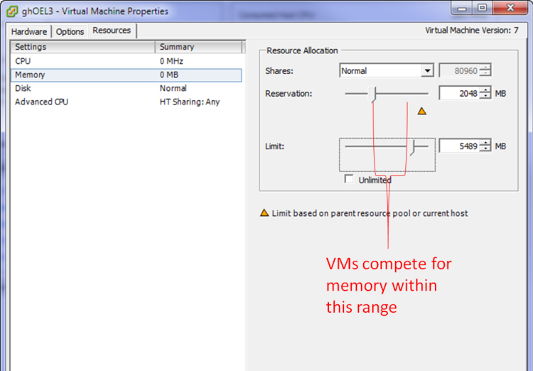
As with memory,  ESX uses reservations, shares and limits to determine which virtual CPUs get to use the physical CPUs if the total virtual demand exceeds physical capacity.

• Shares represent the relative amount of CPU allocated to a VM if there is competition.  The more shares the relatively larger number of CPU cycles will be allocated to the VM. All other things being equal, a VM with twice the number of shares will get access to twice as much CPU capacity.
• The Reservation determines the minimum amount of CPU cycles allocated to the VM
• The Limit determines the maximum amount of CPU that can be made available to the VM

VMs compete for CPU cycles between the limit and their reservation.  The outcome of the competition is determined by the relative number of shares allocated to each VM.

 

Measuring CPU consumption in a virtual machine

Because ESX can vary the amount of CPU actually allocated to a VM, operating system reports of CPU consumption can be misleading.  On a physical machine with a single 2 GHz CPU, 50% utilization clearly means 1GHz of CPU consumed.  But on a VM, 50% might mean 50% of the reservation, the limit, or anything in between.  So interpreting CPU consumption requires the ESX perspective as to how much CPU was actually provided to the VM.

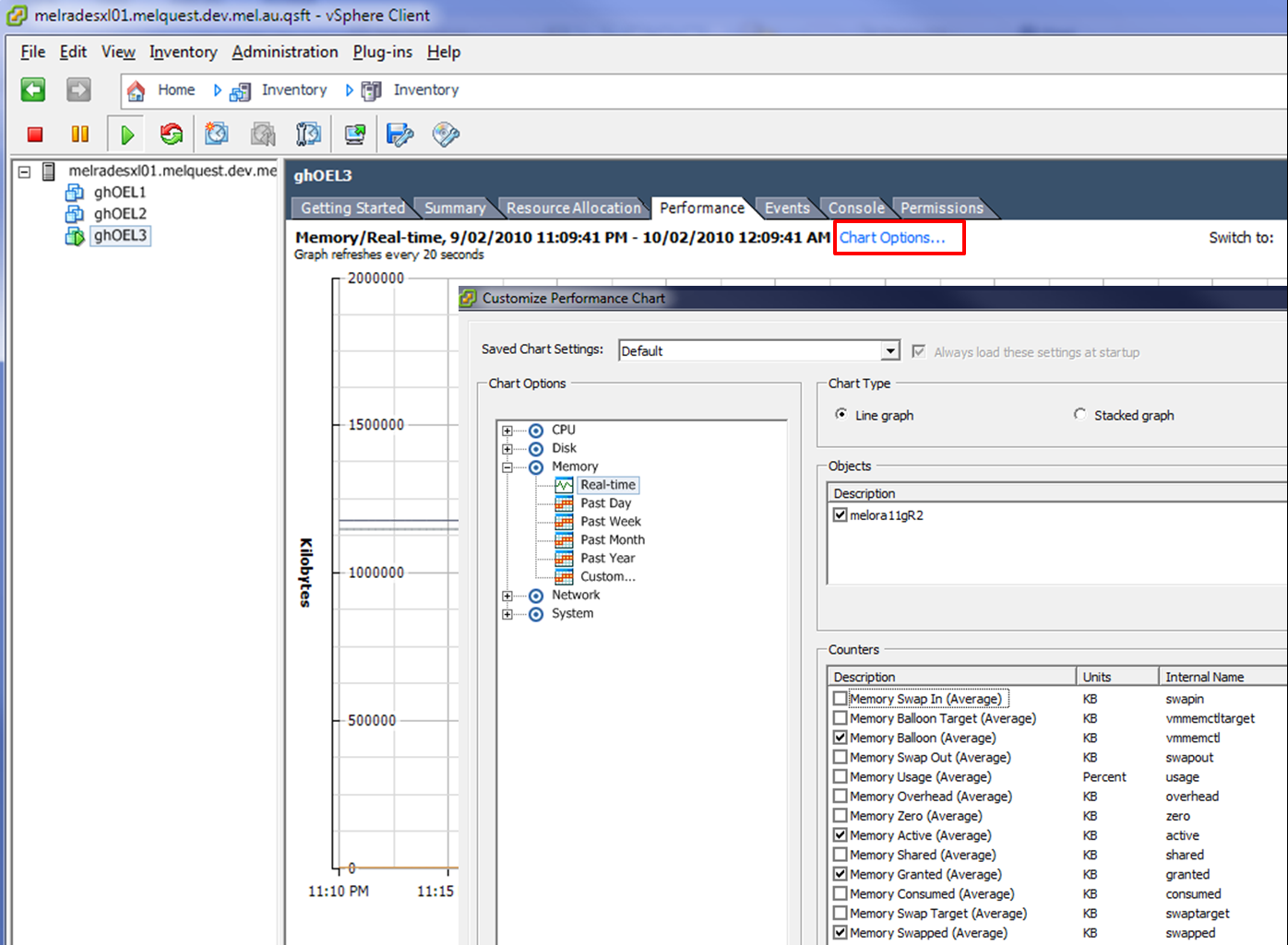
The Performance monitor in the vSphere client gives us the traditional measures of CPU consumption:  CPU used, CPU idle, etc.  However it adds the critical “CPU Ready” statistic.  This statistic reflects the amount of time the VM wanted to consume CPU, but was waiting for a physical CPU to become available.  It is the most significant measure of contention between VMs for CPU power.

For instance in the chart below, we can see at times that the amount of ready time is sometimes almost as great as the amount of CPU actually consumed.  In fact you can probably see that as the ready time goes up, the VMs actual CPU used goes down – the VM wants to do more computation, but is unable to do so due to competition with other VMs.

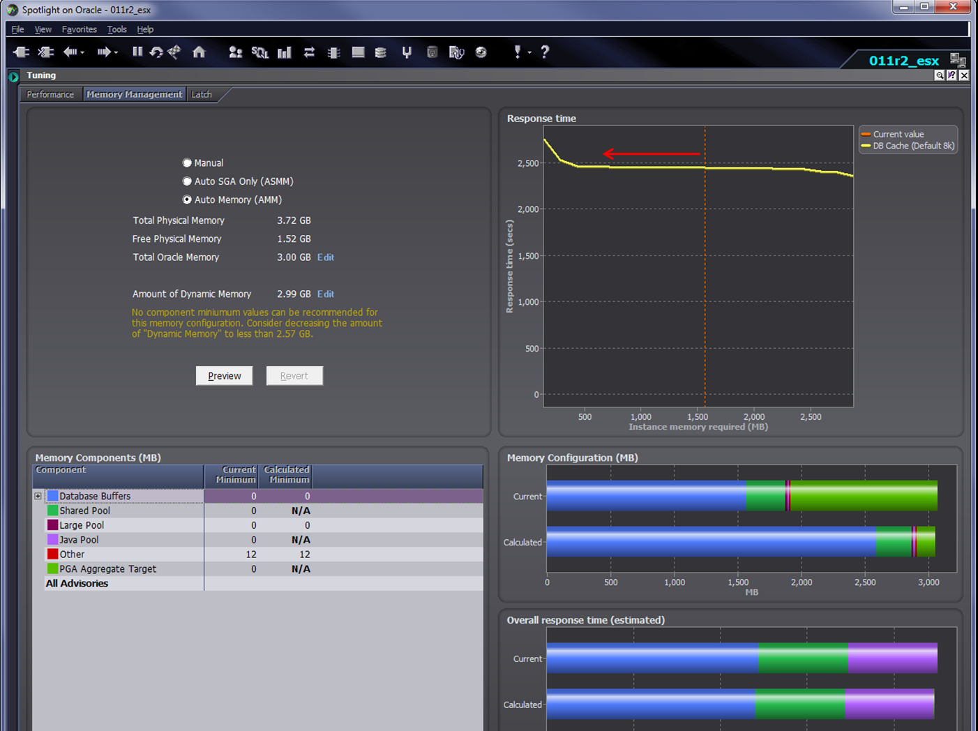
The display of milliseconds in each mode makes it hard to work out exactly what is going on.  In the next release of Spotlight on Oracle (part of the Toad DBA suite) we’ll be showing the amount of ready time as a proportion of the maximum possible CPU, and provide drilldowns that show CPU limits, reservations, utilization and ready time. 

Co-scheduling

For a VM with multiple virtual CPUs, ESX needs to synchronize vCPUs cycles with physical CPU consumption.   Significant disparities between the amounts of CPU given to each vCPU in a multi-CPU VM will cause significant performance issues and maybe even instability.    A “strict co-scheduling policy” is one in which all the vCPUs are allocated to the physical CPUs simultaneously, or at least when any one CPU falls significantly behind in processing.   Modern ESX uses “relaxed co-scheduling” in which only CPUs that have fallen behind need to be scheduled.

In practice however,  on a multi-CPU system all the CPUs generally consume roughly equivalent amounts of CPU and most of the time all of them will need to be scheduled together.  This can make it harder for ESX to allocate CPUs.   For instance, in the diagram below we see how the more vCPUs are configured, the fewer scheduling choices are available to the ESX scheduler:

(Thanks to Carl Bradshaw for letting me reprint that diagram from his Oracle on VMWare whitepaper)

As a result,  you can actually find performance decreasing as the number of cores increases.  This will be most apparent if you try and configure as many vCPUs as physical CPUs. 

Even if there is no competition from other virtual machines, the ESX hypervisor itself will require CPU resources and find it difficult to schedule all the cores of the VM.  This is very noticeable on VMware workstation:  if you create a two-CPU virtual machine on a dual core laptop, it will almost certainly perform worse than a single CPU VM, because VMware will have trouble scheduling both the vCPUs simultaneously.

In general, don’t allocate a lot of vCPUs unless you are sure that the ESX server is usually under light load from other VMs and that your database actually needs the extra cores.

Summary

Effective ESX memory configuration requires co-ordination between Oracle’s memory management and the ESX memory management to avoid PGA or SGA ending up on disk.  CPU is a lot simpler.  In general I recommend the following:

• Avoid over-allocating CPU cores:  don’t automatically assume that more CPUs will lead to better performance
• Use reservations, limits and shares to determine the relative amount of CPU that will be allocated to your VM
• Monitor the ESX “CPU ready” statistic to determine how competition with other VMs is affecting your virtualized databases’ access to CPU.

Memory Management for Oracle databases on VMWare ESX

The trend towards virtualization of mid-level computing workloads is progressing rapidly.  The economic advantages of server consolidation and the – often exaggerated – reduction in administration overheads seem pretty compelling.  And virtualized servers are quicker to provision and offer significant advantages in terms of backup, duplication and migration.

The virtualization of Oracle databases has proceeded more slowly, due to concerns about performance, scalability and support.  Oracle corporation has given mixed messages about support for virtualized databases,  though they currently appear to have conceded that Oracle databases on VMWare are supported, at least for single instance databases (see ).

Oracle would prefer that we use their Xen-based virtualization platform, but they face an uphill battle to persuade the data centers to move from ESX, which is established as a defacto platform in most sites.

So like it or not, we are probably going to see more databases running on ESX and we’d better understand how to manage ESX virtualized databases.  In this post, I’m going to discuss the issues surrounding memory management in ESX.

Configuring memory

When creating a VM in ESX we most significantly configure the amount of “physical” memory provided to the VM.  If there is abundant memory on the ESX server then that physical memory setting will be provided directly out of ESX physical memory.  However, in almost all ESX servers the sum of virtual memory exceeds the physical ESX memory and so the VM memory configuration cannot be met.  The Resources tab options control how VMs will compete for memory.

The key options are:

• Shares.  These represent the relative amount of memory allocated to a VM if there is competition.  The more shares the relatively larger the memory allocation to the VM. All other things being equal, a VM with twice the number of shares will get twice the memory allocation.  However, ESX will “tax” memory shares if the VM has a large amount of idle memory. 
• Reservation:  This is the minimum amount of physical memory to be allocated to the VM.  If there is insufficient memory to honor the reservation then the VM will not start. 
• Limit:  This is the maximum amount of memory that the VM will use.   The advantage of using limit rather than simply reconfiguring the VM memory is that you don’t need to reboot the VM to adjust the memory limit.

So in general, an ESX VM will have a physical memory allocation between the reservation and the limit.  In the event that VMs are competing for memory, the shares setting will determine who gets the most memory.

Ballooning and Swapping

When ESX wants to adjust the amount of physical memory allocated to the VM, it has two options:

• If VMWare tools are installed, ESX can use the vmmemctl driver (AKA the “balloon” driver) which will force the VM to swap out physical memory to the VMs own swapfile.
• If VMWare tools are not installed, then ESX can directly swap memory out to it’s own swapfile.   This swapping is “invisible” inside the VM.

Let’s look at these two mechanisms.  Let’s start with a VM which has all it’s memory mapped to ESX physical memory as in the diagram below:

Life is good – VM physical memory is in ESX physical memory, which is generally what we want. 

If there is pressure on ESX memory and ESX decides that it wants to reduce the amount of physical memory used by the VM – and VMWare tools is installed – then it will use the vmmemctl driver.  This driver is also refered to as the “balloon” driver – you can think of it expanding a balloon within VM memory pushing other memory out to disk. This driver will – from the VMs point of view – allocate enough memory within the VM to force the VM Operating System to swap out existing physical memory to the swapfile.   Although the VM still thinks the vmmemctl allocations are part of it’s physical memory address space, in reality memory allocated by the balloon is available to other VMs:

Inside the VM, we can see that memory is swapped out by using any of the standard system monitors:

 

If VMware tools are not installed, then ESX will need to swap out VM memory to it’s own swap file.  Inside the VM it looks like all of the memory is still allocated, but in reality some of the memory is actually in the ESX swap file.

 

Monitoring memory

We can see what’s going on in the ESX server by using the Performance monitoring chart.  Personally, I like to customize the chart to show just active memory, granted memory, balloon size and swap size as shown below:

 

Recommendations for Oracle databases

Hopefully we now have some idea how Oracle manages ESX memory and how the physical memory in the VM can be reduced.

Its true that for some types of servers – a mail or file server for instance – having physical memory removed from the VM might be appropriate and cause only minor performance issues.  However, for an Oracle database, any reduction in the physical memory of the VM is probably going to result in either SGA or PGA memory being placed on disk.  We probably never want that to happen.

Therefore, here are what I believe are the ESX memory best practices for Oracle databases:

• Use memory reservations to avoid swapping.  There’s no scenario I can think of in which you want PGA and SGA to end up on disk, so you should therefore set the memory reservation to prevent that from happening.  
• Install VMware tools to avoid “invisible” swapping.  If VM memory ends up on disk you want to know about it within the VM.  The vmmemctl “balloon” driver allows this to occur.  Furthermore, the OS in the VM probably has a better idea of what memory should be on disk that ESX.  Also, if you use the vmmemctl driver then you can use the LOCK_SGA parameter to prevent the SGA from paging to disk.    
• Adjust your Oracle targets and ESX memory reservation together.  For instance, if you adjust MEMORY_TARGET in an 11g database, adjust the ESX memory reservation to match.  Ideally,  the ESX memory reservation should be equal to MEMORY_TARGET plus some additional memory for the OS kernel, OS processes and so on.   You’d probably want  between 200-500MB for this purpose.
• Don’t be greedy.  With physical servers we are motivated to use all the memory we are given.  But in a VM environment we should only use the memory we need so that other VMs can get a fair share.  Oracle advisories – V$MEMORY_TARGET_ADVICE, V$SGA_TARGET_ADVICE, V$PGA_TARGET_ADVICE – can give you an idea of how performance would change if you reduced – or increased – memory.  If these advisories suggest that you can reduce memory without impacting performance then you may wish to do so to make room for other VMs. 

In the next release of Spotlight on Oracle, we will be monitoring ESX swapping and ballooning and raising alarms if it looks like ESX is pushing PGA or SGA out to disk.  Spotlight also has a pretty good – if I do say so myself – memory management module that can be used to adjust the database memory to an optimal level (see below).  In a future release I hope to enhance that capability to allow you to adjust database and ESX reservations in a single operation.  

 

Flash tablespace vs. DB Flash Cache

In this post I'm going to report on some performance comparisons I've recently conducted on using SSD flash storage for datafiles vs. using the new Oracle 11GR2 database flash cache.  

It sometimes seems like I’ve been waiting for the the end of the spinning magnetic disk all my professional  life.   The technology is so ancient, so clearly limited and (argh) mechanical.  So the fact that Solid State Disk (SSD) is becoming more an more practical as a database storage medium - and directly supported by Oracle in 11GR2 - is very exciting.  

Using SSD as part of database storage can certainly yield big results, but it's important to understand the performance characteristics of flash SSD and make sure we don't use it inappropriately. 

SSD comes in two flavours:

• Flash  based SSD uses the familiar flash technology that underlies the ubiquitous USB drives that have replaced floppy disks for small portable data storage.   Flash RAM is cheap, provides permanent storage without battery backup and so has low power consumption. 
• DDR RAM based SSD uses memory modules that are not particularly different in nature from those that provide core memory for the server.   This RAM is backed by non-volatile storage (disk or flash RAM) and internal batteries.  In the event of a power failure, the batteries provide enough power to write the RAM memory to the non-volatile storage.  

DDR SSD is too expensive (in terms of $$/GB) to be very useful to we database professionals today.  But Flash based disk is becoming an increasingly viable alternative to magnetic disk.

Read, write and erase operations

Flash disk storage is organized into pages – typically 4K – and blocks – typically 256K.  For read operations, the flash disk can return data very quickly from individual pages.  Writing to a page is slower – maybe 10 times slower.  However,  it is only possible to write a page of data if there is an empty page in the block.   If we need to write to a full block, it must first be erased.   The Wikipedia entry on SSD gives the following figures for seek, write and erase times:

 

As a flash SSD fills with data, the percentage of simple block level writes that require an erase increases, and the write performance of the flash SSD degrades.

The TRIM API function

High end flash SSD support an API call TRIM, which allows the OS to proactively erase full blocks so that writes can complete with only a page-level IO.  Most high end drives also support wear-leveling algorithms that move hot-pages around the device to avoid the risk of block level failures.  Flash drives can only support a limited number of erase operations before a block becomes unreliable,  but this is minimized providing the disk automatically moves hot pages around in physical storage. 

MLC vs SLC

Cheap flash drives generally use Multi-Level-Cell (MLC) technology in which each cell can store two bits of data rather than SLC which can only store one bit.  The effect of MLC is to increase density at the expense of performance, particularly write performance.   MLC is also less reliable in terms of data loss. If you’re concerned about write performance – and you probably should be – then you should avoid MLC.  

In general,  if you want a high performance flash SSD - and why get one if it's not high performance - you should go for a SLC based flash SSD that supports the TRIM API and has good wear leveling capabilities.  For my testing,  I used an Intel X-25 E 32GB drive.   It cost about $600 Australian (about $534 US dollars).

The problem with read/write speed disparities

Given that most databases do many more reads than writes, do we need to worry about the disparity between seek times and write times for flash SSD?  The answer is definitely YES.   For an Oracle database, a big mismatch between the ability to read from a device and the ability to write to the device can be particularly harmful when performing transactional activity through the buffer cache.

The issue relates to the caching of data within the buffer cache.  If it’s very much easier to put blocks into the buffer cache than to write them out, then there’s a good chance that the buffer cache will fill up with dirty (unmodified) blocks and that free buffer waits will result.  The figure below illustrates how free buffer waits can occur:

 

(This illustration from Oracle Performance Survival Guide).

If you're using cheap flash drives, then the write speed is going to be much slower than the read speed and consequently you could end up with free buffer waits becoming your limited factor during high transactional activity. 

Enter the Oracle Database Flash Cache 

Oracle's database flash cache provides an alternative way of exploiting flash SSD.  Instead of putting the entire datafile on flash, we use flash as a secondary cache.  The flash cache can be massive and can speed up reads for frequently accessed blocks.  But if the flash drive is busy, Oracle will simply decline to write to the cache.  That way we can get some of the advantage of flash for read optimization without having to pay the write penalty.  

I outlined the flash cache algorithms in this previous post, and here's the diagram I used there to outline the lifecycle of a block when the database flash cache is enabled:

The important part of this architecture is that the DBWR will only write the block to the flash cache if it is not overloaded.  If the DBWR gets busy, then the flash cache write can be omitted and while this will reduce the efficiency of the cache, it prevents the buffer cache from filling up with modified blocks - so free buffer waits should not result. 

Flash disk read performance

Let's see how this pans out in practice.  Below we see the relative performance for 500,000 random indexed reads against:

1. A table on magnetic disk with no flash cache
2. A table on magnetic disk with flash caching
3. A table stored directly on flash disk 

The magnetic disk was a Seagate 7200.7 80GB Barracuda drive, while the Solid State Disk drive was an Intel X-25 E 32GB drive which is a pretty high end SLC drive.  In both cases, the tablespaces were created on raw partitions to avoid filesystem caching and the redo logs and other tablespaces were on a seperate drive.   The database was restarted prior to each test. 

Here's the read performance:

 

As you'd expect,  storing the table directly on flash is fastest, since there are only read I/Os, and every read I/O is from the much faster flash SSD.   Note that the flash cache gives us a lot of advantages as well - the number of database file IOs is reduced, and the reads from the flash cache are very fast indeed. 

Update performance

Next I measured the performance of primary key based UPDATEs.  The performance for such an UPDATE is a mix of read time - get the block into cache - and DBWR performance.  If the DBWR can't write the modified blocks out fast enough then free buffer waits and/or write complete waits will occur. 

What I expected was that the flash tablespace test would show a lot of free buffer waits, since in theory flash writes are so much slower than flash reads.  I thought that using the flash cache would avoid that issue, and provide the best performance.   However, the results surprised me:

I repeated the above tests about a dozen times with a variety of workloads, but the results were pretty similar in every case.  While using the flash cache is better than no flash at all, it's still better to put the table directly on flash storage.   The X-25 E was simply able to sustain a write rate much higher than I had expected - about 2,000 writes/sec.   Intel claim - and now I believe - that they have sophisticated algorithms that avoid the write penalty usually associated with the flash SSD storage medium.

Note that it's actually the Flash Cache configuration that generates the most free buffer waits.  The flash cache allows Oracle to achieve much higher logical read rates but - since the writes still go to the relatively slower spinning magnetic disk - the buffer cache often fills with dirty blocks. 

It may be that over time the performance of the X-25 will reduce when all the blocks have been written to at least once  Erase operations become more prevalent.   However,   if the TRIM API is working properly then this degradation should in theory be avoided.  Note that TRIM support is not universal - not all SSDs and older versions of Windows may not support it. 

Write complete waits: flash cache

In previous postings I noted that the DBWR will skip writing to the flash cache when busy, which should prevent flash cache activity being a direct cause of buffer busy waits.   However,  I noticed under some workloads that I would get a large number of "write complete waits: flash cache".  For instance, the output below shows about 74% of elapsed time in this wait:

Write complete waits occur when a session wants to modify a block, but the DBWR is in the process of writing it out to the datafile.  The flash cache equivalent occurs for the same reason, but instead of writing it to the datafile, the DBWR is writing it to the flash cache.  This phenomenon can occur when individual blocks are being modified at very high rates;  in this scenario, the chance that the block will be modified before the DBWR writes it out can be substantial. 

Conclusion

I'm very impressed with the performance of the X-25 E flash SSD drive.  If it can maintain it's high write throughput over time, then it offers a significant increase in throughput over traditional spinning disk or over the new 11GR2 database flash cache.  However, a few words of warning:

• I did not stress test the disk over a long period of time.  Some flash drives exhibit more write latency as they wear in.  In theory, the TRIM functionality of the Intel X-25 E should avoid that, but I did not verify it in these tests.
• Flash drives can be an unreliable form of storage over long periods of time.  Any disk can fail of course, but if you run a flash disk hot it will likely fail before a magnetic disk (though it will do more work during that period). 
• In my tests, my table was small enough to fit on the flash storage.  Had it not, then using the database flash cache would have allowed me to get some benefits from the flash drive without having to buy enough storage to fit the whole database on the SSD.

I'm now even more enthusiastic about the use of flash drives.  Providing you buy a high-performance drive (think SLC & TRIM) then you could consider placing entire tablespaces or database on these drives.  If you can't afford top end flash drives for all your data, then the 11GR2 database flash cache can give you a pretty substantial performance boost. 

Best practices with Python and Oracle

This is the third in a series of postings outlining the basics of best practices when coding against Oracle in the various languages.  In Oracle Performance Survival Guide (and in it's predecessor Oracle SQL High Performance Tuning) I emphasise the need to use bind variables and array processing when writing Oracle programs.   The book provides examples of both in PL/SQL and Java, while these postings outline the techniques in other languages. 

Previous postings covered .NET languages and perl. 

The Python code for the examples used in the posting is here. 

I became interested in python a few years back when I read the article Strong Typing vs Strong Testing in Best Software Writing and from various other sources that sjggested that Python was a more modern and robust scripting language than Perl (and superior to Java for that matter).  I dabbled with Python and thought about dropping perl as my scripting language of choice but in the end stuck with perl and Java as my primary languages because: (a) decades of perl experience were going to be too hard to replicate in Python and (b) the database drivers for python were not universally of the same quality as perl.

Nevertheless,  Python is an excellent language for Oracle development and utilities and the cx_oracle driver fully supports best coding practices for Oracle. 

Bind Variables

As with most languages, it's all too easy to concatenate literals - creating a unique SQL which mush be re-parsed - rather than using the more efficient bind variable approach.  If anything, it's even easier in Python, since Python's string substitution idiom looks very similar to bind variables.  

For instance, in this fragment, the "%d" literal in the SQL text represents the substitution value for the query:

 

Of course, if you are at all familiar with Python you'll know that the "%" operator substitutes the values in the subsequent list into the preceding string - so this example creates many unique SQL statements leading to high parse overhead; and possibly to library cache latch or mutex contention.  

The cursor execute method allows you to specify bind variables as a list following the SQL, as in this example:

In line 129 we define a named bind variable ":x_value".  Within the execute procedure (line 130) we assign the bind variable to the value of the python variable "i". 

There's a couple of different styles of using bind variables in python.  You can use positional parameters (eg ":1",":2", etc) and pass in a python list that contains the values in sequence and - as we shall see soon - you can bind arrays.  

As with any programming language, using bind variables improves performance by reducing parse overhead and library cache latch or mutex contention.  The above SQL is about as simple as you can get, so parse overhead reductions should be modest.   As the only active session on my (local laptop) database,  library cache contention would not be expected either.  Nevertheless,  elapsed time even in this simple example reduced by more than 1/2 when bind variables were used. 

Array Fetch

Fetching rows in batches generally reduces elapsed time for bulk selects by up to a factor of 10.  Array fetch works to improve performance by reducing network round trips and by reducing logical reads.

Like most modern interfaces,  Python with cx_oracle will do some level of array fetch for you, even if your program handles rows and at a time.  So in the example below, it looks like we are fetching rows one at a time:

Using SQL trace, we can see that Python in fact fetched rows in batches of 50 (this is shown using Spotlight on Oracles trace file analyzer, but you can deduce the same thing from tkprof output): 

You can adjust or view the array size through the arraysize cursor property.  Here we foolishly set the arraysize to 1:

Python provides fetchmany() and fetchall() calls in addition to the "fetchone" call used above.  While these do affect the handling of the result set on the python side, the arraysize variable continues to control the size of the array fetch actually sent to Oracle.   The fetchall() call is more efficient in some ways, but requires that you have enough memory on the client side to hold the entire result set in memory:

 

 Fetchmany() let's you handle the results in batches:

The arraysize cursor property determines how many rows are in each set, so with fetchmany() the python code corresponds most closely to the underlying Oracle processing logic. 

For 500,000 rows, here's the performance of each of the approaches we've tried so far:

 

Although fetchall() performed best in this example, it may backfire for very massive result sets, because of the need to allocate memory for all of the data in the result set.   fetchmany() may be the best approach if you're not sure that the result set is small enough to fit comfortably in memory. 

Array insert

Array insert has similar performance implications as array fetch, but it harder to program and does not happen automatically.  The "natural" way to perform inserts is probably to loop through the rows and assign them one at a time:

The values to be inserted are supplied as a Python list which is bound to the positional bind variables (":1, :2") defined in the SQL.   In this example we used the prepare method to create the SQL once before executing it many times.  This is not a bad practice, but doesn't seem to have any impact on parse overhead:  Python only reparses the SQL when the SQL text changes.

To perform an array insert, we create a "list of lists" which defines our array to be inserted.  We then call the executemany() method to insert that array:

Each entry in the arrayValues list is itself a list that contains the values to be bound.

As usual, the performance improvements are fairly remarkable.  The chart above compares the time to insert 500,000 rows using array insert vs. single row inserts. 

Conclusion

The basics of good practice in Python when working with an Oracle database are much the same as those for other languages:

• Use bind variables whenever possible
• Array fetch is performed automatically, but you can tweak it to get better performance
• Array insert requires manual coding but is definitely worth it

Histograms of histograms

One of our TOAD customers asked us if we could show a chart of CBO histogram values so that they could observe the skew in column values.   We don't currently, but will in an upcoming version of SQL Optimizer (part of TOAD DBA and Developer suites).  In the meantime, the idea of have an SQL that generated a histogram (as bar charts are sometimes called) of a histogram seemed appealing, so here's some SQL to do that. 

In case you don't know,  Oracle uses height balanced histograms when the number of distinct values is high.  In a height balanced histogram the number of rows in each bucket is about the same, but the range of values in each bucket varies.  However, when the number of buckets in the histogram is greater than or equal to the number of distinct column values then Oracle will create a frequency histogram. In a frequency histogram each bucket represents a value, and the number of rows matching the value is recorded.  The Oracle documentation set describes the two types of histograms here. 

This script will create a bar chart (AKA a histogram) as for a frequency histogram.  For instance, here is a display of the values for the CUST_DATE_OF_BIRTH column in the CUSTOMERS table:

The script uses the ENDPOINT_ACTUAL_VALUE column if present, otherwise the ENDPOINT_VALUE column.  For numeric columns,  ENDPOINT_VALUE is fine,  but for character columns it's meaningless.   

Unfortunately ENDPOINT_ACTUAL_VALUE is not generally populated.  According to Jonathan Lewis in Cost Based Oracle Fundamentals,  from 9i onwards:  "Oracle only populates the endpoint_actual_value column of the histogram views if there is at least one pair of values that, roughly speaking, are identical for the first six characters".

So for most character columns, the script will report something unhelpful like this (this is the CUSTOMERS.CUST_INCOME_LEVEL column):

Tom Kyte provided a PL/SQL function "hexstr" that can decode the ENPOINT_VALUE to a character string - at least for the first 6 bytes.  So using Tom's function, we can get a better sense of the distribution of CUST_INCOME_LEVEL:

Remember, these "histogram histograms" are only really useful for FREQUENCY histograms;  check USER_TAB_COL_STATISTICS to see what types of histograms exist on your columns:

Also the accuracy of the histograms is going to vary depending on your DBMS_STATS options and on how recently you collected the statistics.  All that having been said, the query may be a good way to get a quick idea of how your data is distributed which can be critical when tuning SQL.